Results

Every Starsim simulation produces results: time series of quantities such as the number of infections, deaths, or people in each disease state. This page explains how results are organized, how to access and manipulate them, and how to plot and export them.

Where results live

After a sim has run, all of its outputs are stored in sim.results, which is a nested structure. Each module adds its own group of results, and there are also some sim-level results (such as n_alive):

import starsim as ss
ss.options(jupyter=True)

sim = ss.Sim(n_agents=2000, diseases='sir', networks='random', verbose=0).run()

# Top-level groups: one per module, plus sim-level results
print('Result groups:', list(sim.results.keys()))

# The results within the SIR disease module
print('SIR results:  ', list(sim.results.sir.keys()))

Result groups: ['timevec', 'randomnet', 'sir', 'n_alive', 'n_female', 'new_deaths', 'new_emigrants', 'cum_deaths']
SIR results:   ['timevec', 'n_susceptible', 'n_infected', 'n_recovered', 'prevalence', 'new_infections', 'cum_infections']

You access an individual result by drilling down through the module name:

new_infections = sim.results.sir.new_infections
print(new_infections)

Result(SIR.new_infections: min=0, mean=38.902, max=382)

Anatomy of a result

Each result is an ss.Result object. It behaves like a NumPy array (so you can index, slice, and do arithmetic on it directly), but it also carries metadata:

Attribute	Meaning
`values`	The underlying NumPy array of values
`timevec`	The time points corresponding to each value
`label`	A human-readable label (used in plots)
`scale`	Whether the quantity scales with population size (e.g. a count)
`low`, `high`	Optional uncertainty bounds (populated by `MultiSim.reduce()`)

res = sim.results.sir.new_infections

# Use it like an array
print(f'Peak new infections: {res.max():.0f}')
print(f'Total infections:    {res.sum():.0f}')
print(f'Final timestep:      {res[-1]:.0f}')

# ...but it also knows its own time axis and label
print(f'Label:    {res.label}')
print(f'First date: {res.timevec[0]}')

Peak new infections: 382
Total infections:    1984
Final timestep:      0
Label:    New infections
First date: 2000.01.01

Plotting results

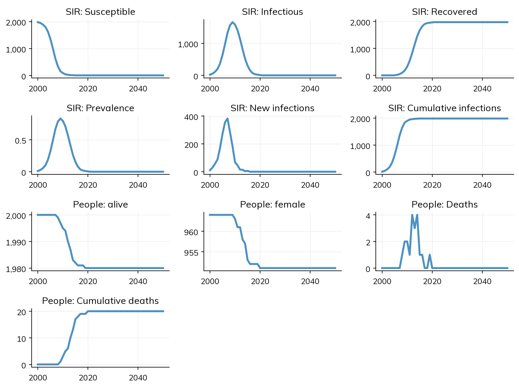
The quickest way to see everything is sim.plot(), which plots all results flagged for automatic plotting:

sim.plot()

Figure(896x672)

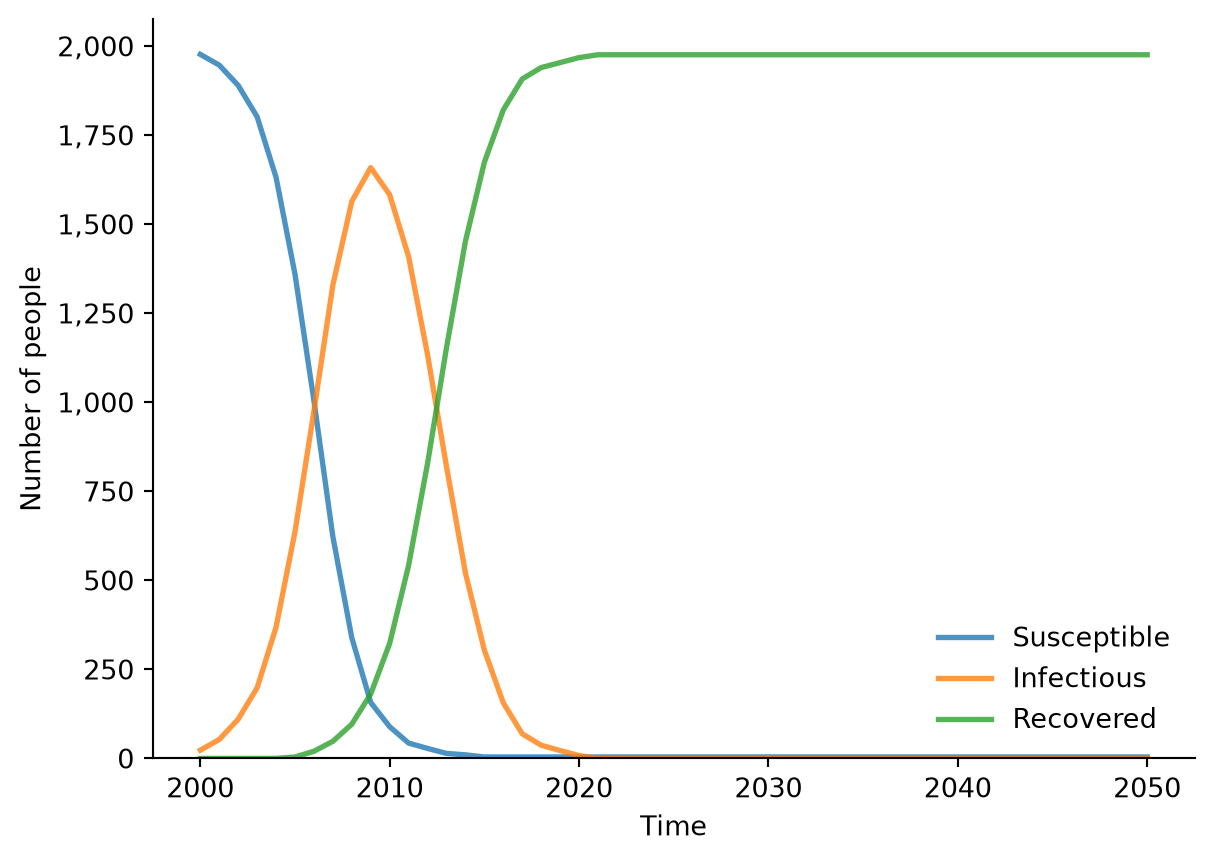
You can plot a single module’s results, or even a single result on its own:

# Just the SIR results
sim.diseases.sir.plot()

Figure(672x480)

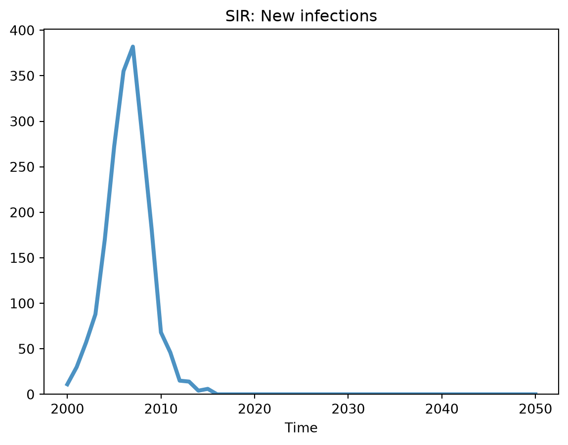
# A single result, with its label and time axis handled automatically
sim.results.sir.new_infections.plot()

Figure(672x480)

Exporting results

To get results into a pandas dataframe — for example, to save to CSV or analyze further — use to_df(). This works at the level of a single module:

df = sim.results.sir.to_df()
df.head()

	timevec	n_susceptible	n_infected	prevalence	new_infections	cum_infections
0	2000-01-01	1977.0	23.0	0.0115	11.0	11.0
1	2001-01-01	1947.0	53.0	0.0265	30.0	41.0
2	2002-01-01	1890.0	110.0	0.0550	57.0	98.0
3	2003-01-01	1802.0	198.0	0.0990	88.0	186.0
4	2004-01-01	1632.0	368.0	0.1840	170.0	356.0

or for the whole sim at once, which flattens every module’s results into one wide dataframe:

df = sim.to_df()
print('Columns:', list(df.columns))
df.head()

Columns: ['timevec', 'randomnet_n_edges', 'sir_n_susceptible', 'sir_n_infected', 'sir_n_recovered', 'sir_prevalence', 'sir_new_infections', 'sir_cum_infections', 'n_alive', 'n_female', 'new_deaths', 'new_emigrants', 'cum_deaths']

	timevec	randomnet_n_edges	sir_n_susceptible	sir_n_infected	sir_prevalence	sir_new_infections	sir_cum_infections	n_alive	n_female
0	2000-01-01	10000.0	1977.0	23.0	0.0115	11.0	11.0	2000.0	964.0
1	2001-01-01	10000.0	1947.0	53.0	0.0265	30.0	41.0	2000.0	964.0
2	2002-01-01	10000.0	1890.0	110.0	0.0550	57.0	98.0	2000.0	964.0
3	2003-01-01	10000.0	1802.0	198.0	0.0990	88.0	186.0	2000.0	964.0
4	2004-01-01	10000.0	1632.0	368.0	0.1840	170.0	356.0	2000.0	964.0

If you’d rather have a flat dictionary of results keyed by module_result (rather than a dataframe), use sim.results.flatten().

Results across multiple runs

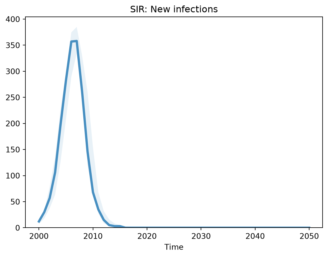
When you run many sims with ss.MultiSim, you usually want summary statistics across the runs rather than each run individually. Calling reduce() (or the convenience methods mean() / median()) combines the runs and populates the low and high uncertainty bounds on each result:

msim = ss.MultiSim(ss.Sim(n_agents=2000, diseases='sir', networks='random', verbose=0), n_runs=5)
msim.run()
msim.reduce()

# After reducing, each result carries low/high bounds, which plot() shows as a band
res = msim.results['sir_new_infections']
print(f'Bounds available: low={res.low is not None}, high={res.high is not None}')
res.plot()

Bounds available: low=True, high=True
Figure(672x480)

Note that across multiple runs the results are stored in a flattened structure keyed by module_result (e.g. sir_new_infections), so you access them with msim.results['sir_new_infections'] rather than the nested msim.results.sir... form used for a single sim.

Adding your own results

Any module can define custom results. For one-off analyses, the simplest approach is an Analyzer; to bake results into a module you’re writing, define them with self.define_results() (see Adding new modules). Either way, your results are stored in sim.results alongside the built-in ones and are exported by to_df() automatically.