Calibration using Optuna-Starsim integration

Disease models typically require contextualization to a relevant setting of interest prior to addressing “what-if” scenario questions. The process of tuning model input parameters so that model outputs match observed data is known as calibration. There are many approaches to model calibration, ranging from manual tuning to fully Bayesian methods.

For many applications, we have found that an optimization-based approach is sufficient for initial exploration. Such methods avoid the tedious process of manual tuning and are less computationally expensive than fully Bayesian methods. One such optimization-based approach is the Optuna library, which is a Bayesian hyperparameter optimization framework. Optuna is designed for tuning hyperparameters of machine learning models, but it can also be used to calibrate disease models.

Calibration libraries often treat the disease model as a black box, where the input parameters are the “hyperparameters” to be tuned. The calibration process is often iterative and requires a combination of expert knowledge and computational tools. The optimization algorithm iteratively chooses new parameter values to evaluate, and the model is run with these values to generate outputs. The outputs are compared to observed data, and a loss function is calculated to quantify the difference between the model outputs and the observed data. The optimization algorithm then uses this loss function to update its search strategy and choose new parameter values to evaluate. This process continues until the algorithm converges to a set of parameter values that minimize the loss function.

While many optimization algorithms are available, Starsim has a built-in interface to the Optuna library, which we will demonstrate in this guide. We will use a simple Susceptible-Infected-Recovered (SIR) model as an example. We will tune three input parameters, the infectivity parameter, beta, the initial prevalence parameter, init_prev, and the Poisson-distributed degree distribution parameter, n_contacts. We will calibrate the model using a beta-binomial likelihood function so as to match prevalence at three distinct time points.

For a comparison of optimization-based and Bayesian approaches to calibration, see the SIR calibration workflows notebook.

We begin with a few imports and default settings:

# Notebook configuration
%load_ext autoreload
%autoreload 2
%matplotlib inline

##%% Imports and settings
import sciris as sc
import starsim as ss
import numpy as np
import pandas as pd

n_agents = 2e3
debug = False # If true, will run in serial

The calibration class will require a base Sim object. This sim will later be modified according to parameters selected by the optimization engine. The following function creates the base Sim object.

def make_sim():
    sir = ss.SIR(
        beta = ss.perday(0.075),
        init_prev = ss.bernoulli(0.02),
    )
    random = ss.RandomNet(n_contacts=ss.poisson(4))

    sim = ss.Sim(
        n_agents = n_agents,
        start = ss.date('2020-01-01'),
        stop = ss.date('2020-02-12'),
        dt = ss.days(1),
        diseases = sir,
        networks = random,
        verbose = 0,
    )

    return sim

Now let’s define the calibration parameters. These are the inputs that Optuna will be able to modify. Here, we define three such parameters, beta, init_prev, and n_contacts.

Each parameter entry should have range defined by low and high as well as a guess values. The guess value is not used by Optuna, rather only for a check after calibration completes to see if the new parameters are better than the guess values.

You’ll notice there are a few other parameters that can be specified. For example, the data type of the parameter appears in suggest_type. Possible values are listed in the Optuna documentation, and include suggest_float for float values and suggest_int for integer types.

To make things easier for the search algorithm, it’s helpful to indicate how outputs are expected to change with inputs. For example, increasing beta from 0.01 to 0.02 should double disease transmission, but increasing from 0.11 to 0.12 will have a small effect. Thus, we indicate that this parameter should be calibrated with log=True.

# Define the calibration parameters
calib_pars = dict(
    beta = dict(low=0.01, high=0.30, guess=0.15, suggest_type='suggest_float', log=True), # Note the log scale
    init_prev = dict(low=0.01, high=0.05, guess=0.15), # Default type is suggest_float, no need to re-specify
    n_contacts = dict(low=2, high=10, guess=3, suggest_type='suggest_int'), # Suggest int just for this demo
)

The optimization engine iteratively chooses input parameters to simulate. Those parameters are passed into the following build_sim function as a dictionary of calib_pars along with the base sim and any other key word arguments. The calib_pars will be as above, but importantly will have an additional key named value containing the value selected by Optuna.

When modifying a sim, it is important to realize that the simulation has not been initialized yet. Nonetheless, the configuration is available for modification at sim.pars, as demonstrated in the function below for the SIR example.

def build_sim(sim, calib_pars, n_reps=1, **kwargs):
    """
    Modify the base simulation by applying calib_pars. The result can be a
    single simulation or multiple simulations if n_reps>1. Note that here we are
    simply building the simulation by modifying the base sim. Running the sims
    and extracting results will be done by the calibration function.
    """

    sir = sim.pars.diseases # There is only one disease in this simulation and it is a SIR
    net = sim.pars.networks # There is only one network in this simulation and it is a RandomNet

    for k, pars in calib_pars.items(): # Loop over the calibration parameters
        if k == 'rand_seed':
            sim.pars.rand_seed = v
            continue

        # Each item in calib_pars is a dictionary with keys like 'low', 'high',
        # 'guess', 'suggest_type', and importantly 'value'. The 'value' key is
        # the one we want to use as that's the one selected by the algorithm
        v = pars['value']
        if k == 'beta':
            sir.pars.beta = ss.perday(v)
        elif k == 'init_prev':
            sir.pars.init_prev = ss.bernoulli(v)
        elif k == 'n_contacts':
            net.pars.n_contacts = ss.poisson(v)
        else:
            raise NotImplementedError(f'Parameter {k} not recognized')

    # If just one simulation per parameter set, return the single simulation
    if n_reps == 1:
        return sim

    # But if you'd like to run multiple simulations with the same parameters, we return a MultiSim instead
    # Note that each simulation will have a different random seed, you can set specific seeds if you like
    # Also note that parallel=False and debug=True are important to avoid issues with parallelism in the calibration
    # Advanced: If running multiple reps, you can choose if/how they are combined using the "combine_reps" argument to each CalibComponent, introduced below.
    ms = ss.MultiSim(sim, iterpars=dict(rand_seed=np.random.randint(0, 1e6, n_reps)), initialize=True, debug=True, parallel=False)
    return ms

# Lets plot a single simulation to see what it looks like
sim = make_sim()
sim.run()
sim.plot()

Figure(768x576)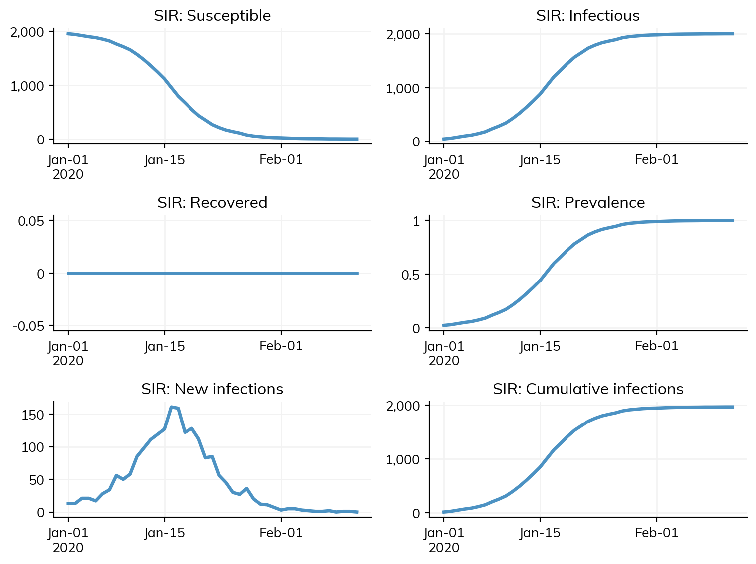

The Starsim framework has been integrated with the Optuna hyperparameter optimization algorithm to facilitate calibration through the Calibration class. Recall that an optimization-based approach to calibration minimizes a function of the input parameters. This function is key to achieving an acceptable calibration.

There are two ways to describe the goodness-of-fit function for the Calibration. The first method is to directly provide a function that the algorithm will call. The eval_fn will be passed each completed sim after running, and is expected to return a float representing the mismatch (lower is better as the optimization algorithm is configured to minimize). Data can be passed into the eval_fn via eval_kwargs.

As an alternative to directly specifying the evaluation function, you can use CalibComponents. Each component includes real data, for example from a survey, that is compared against simulation data from the model. Several components can be used at the same time, for example one for disease prevalence and another for treatment coverage. Each component computes a likelihood of the data given the input parameters, as assessed via simulation. Components are combined assuming independence.

The base class for a component is called CalibComponent, which you can use to define your own likelihood. However, we have provided components for several key likelihood functions including BetaBinomial, Binomial, DirichletMultinomial, GammaPoisson, and Normal. The Normal component is most like a traditional squared error. Each component takes in a name and a weight, which is used when combining log likelihoods.

Importantly, each component takes in the calibration target, the real data that was observed, in an argument called expected. This argument should be a Pandas Dataframe with one row per time point and columns that will depend on the specific component type. For example, the Binomial component requires columns of n (trials) and x (successes).

The components also handle extracting data from each simulation using the extract_fn argument. The value of this argument should be a function that takes in a simulation and returns a Pandas DataFrame. The specifics of the columns will depend a bit on the type of component (e.g. BetaBinomial is different from Normal), but often looks like a simulated version of expected. We will see examples below.

We’ll also see how to use the conform argument, the purpose of which is to temporally align the simulation output to the real data. This argument works along with the extract_fn to produce the final simulation outputs that are used in the likelihood function. The conformer is a function that takes in the expected data you provided and the actual simulation result the comes out of the extract_fn. The conformers we have built in are as follows:

• step_containing: Conform by simply choosing the simulated timestep that contains the time indicated in the real data (expected)
• prevalent: Interpolate the simulated timepoints to estimate the values that would have occurred at each real timepoint
• incident: While the two methods above capture the state of the model at a particular point in time (stocks), this component allows you to capture the behavior of the model over time (flows). Instead of just giving one time value, t, you’ll provide a second time value as well called t1. This conformer will add up events occurring between the two time points.

Let’s make a simple Normal component to capture prevalence at three time points. We’ll use the prevalent conformer to align the simulation output to the real data.

prevalence = ss.Normal(
    name = 'Disease prevalence',
    conform = 'prevalent',

    expected = pd.DataFrame({
        'x': [0.13, 0.16, 0.06],    # Prevalence of infection
    }, index=pd.Index([ss.date(d) for d in ['2020-01-12', '2020-01-25', '2020-02-02']], name='t')), # On these dates
    
    extract_fn = lambda sim: pd.DataFrame({
        'x': sim.results.sir.prevalence,
    }, index=pd.Index(sim.results.timevec, name='t')),

    # You can specify the variance as well, but it's optional (max likelihood estimates will be used if not provided)
    # This could be a single float or an array with the same shape as the expected values
    sigma2 = 0.05, # e.g. (num_replicates/sigma2_model + 1/sigma2_data)^-1
    # Alternatively, specify a variance for each data point
    #sigma2 = np.array([0.05, 0.25, 0.01])
)

Finally, we can bring all the pieces together. We make a single base simulation and create an instance of a Starsim Calibration object. This object requires a few arguments, like the calib_pars and sim. We also pass in the function that modifies the base sim, here our build_sim function. No additional build_kw are required in this example.

We also pass in a list of components. Instead of using this “component-based” system, a user could simply provide an eval_fn, which takes in a completed sim an any eval_kwargs and returns a “mismatch” score to be minimized.

We can also specify the total number of trials to run, the number of parallel works, and a few other parameters.

sc.heading('Beginning calibration')

# Make the sim and data
sim = make_sim()

# Make the calibration
calib = ss.Calibration(
    calib_pars = calib_pars,
    sim = sim,
    build_fn = build_sim,
    build_kw = dict(n_reps=3), # Run 3 replicates for each parameter set
    reseed = True, # If true, a different random seed will be provided to each configuration
    components = [prevalence],
    total_trials = 100, # Use more for a real calibration
    n_workers = None, # None indicates to use all available CPUs
    die = True,
    debug = debug, # Run in serial if True
    verbose = 0,
)

# Perform the calibration
sc.printcyan('\nPerforming calibration...')
calib.calibrate();

—————————————————————

Beginning calibration

—————————————————————





Performing calibration...

[I 2025-10-22 03:13:28,669] A new study created in RDB with name: starsim_calibration

Let’s look at the best parameters that were found. Note that the rand_seed was selected at random, but the other parameters are meaningful.

calib.best_pars

{'beta': 0.010803788895830151,
 'init_prev': 0.04672394969644946,
 'n_contacts': 3,
 'rand_seed': 170396}

Once the calibration is complete, we can compare the guess values to the best values found by calling check_fit.

# Confirm - Note the comparison is here configured over n_reps=15 replicates
sc.printcyan('\nConfirming fit...')

# Increase replicates to 15 for more representative results when running check_fit
calib.build_kw['n_reps'] = 15

calib.check_fit(do_plot=False)

Confirming fit...

Exception ignored in: <_io.BytesIO object at 0x7f38a9c73880>
Traceback (most recent call last):
  File "/home/runner/work/starsim/starsim/starsim/time.py", line 873, in __new__
    def __new__(cls, value=None, base=None, **kwargs):
BufferError: Existing exports of data: object cannot be re-sized
Exception ignored in: <_io.BytesIO object at 0x7f38a9b6b740>
Traceback (most recent call last):
  File "/home/runner/work/starsim/starsim/starsim/time.py", line 873, in __new__
    def __new__(cls, value=None, base=None, **kwargs):
BufferError: Existing exports of data: object cannot be re-sized
Exception ignored in: <_io.BytesIO object at 0x7f38a9b6bc40>
Traceback (most recent call last):
  File "/opt/hostedtoolcache/Python/3.13.7/x64/lib/python3.13/site-packages/dill/_dill.py", line 436, in find_class
    def find_class(self, module, name):
BufferError: Existing exports of data: object cannot be re-sized
Exception ignored in: <_io.BytesIO object at 0x7f38a968e480>
Traceback (most recent call last):
  File "/opt/hostedtoolcache/Python/3.13.7/x64/lib/python3.13/site-packages/pandas/core/internals/blocks.py", line 2789, in new_block
    def new_block(
BufferError: Existing exports of data: object cannot be re-sized
Exception ignored in: <_io.BytesIO object at 0x7f38a9faa340>
Traceback (most recent call last):
  File "/opt/hostedtoolcache/Python/3.13.7/x64/lib/python3.13/site-packages/pandas/core/internals/blocks.py", line 2789, in new_block
    def new_block(
BufferError: Existing exports of data: object cannot be re-sized
Exception ignored in: <_io.BytesIO object at 0x7f3869e5bec0>
Traceback (most recent call last):
  File "<string>", line 0, in <module>
BufferError: Existing exports of data: object cannot be re-sized

Fit with original pars: 6.927809785316569
Fit with best-fit pars: -0.5372379924612117
✓ Calibration improved fit 6.927809785316569 --> -0.5372379924612117

True

After calling check_fit, we can plot the results. This first plot shows the Normal likelihood distributions from each of the 15 simulations we did in check_fit as the colored lines. The vertical dashed line is located at the real (expected) data. Top row is the “guess” values and the bottom row is the new “best” parameters. We want the vertical dashed line to cross the Gaussians at high points, representing high likelihood.

calib.plot()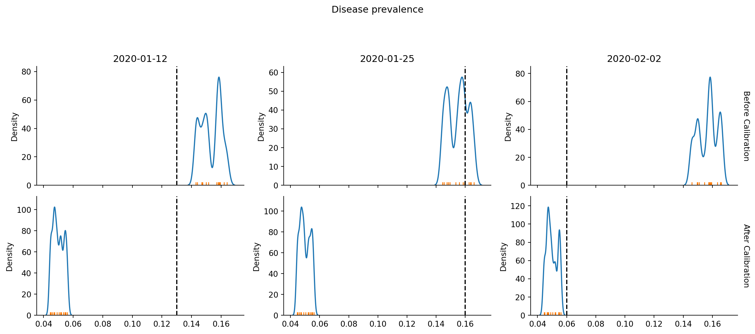

Exception ignored in: <_io.BytesIO object at 0x7f386e1d8c70>
Traceback (most recent call last):
  File "/opt/hostedtoolcache/Python/3.13.7/x64/lib/python3.13/site-packages/seaborn/cm.py", line 1565, in <module>
    _lut_dict = dict(
BufferError: Existing exports of data: object cannot be re-sized

Another way to plot the results is via bootstrapping. Here we repeatedly choose 15 from the n_reps=15 simulations (with replacement), compute the average (or sum for some components), and repeatedly calculate the mean. We then plot the distribution of means, and hope it lands near the vertical dashed lines representing the real data.

calib.plot(bootstrap=True); # Pass bootstrap=True to produce this plot

/home/runner/work/starsim/starsim/starsim/calibration.py:1137: UserWarning: Dataset has 0 variance; skipping density estimate. Pass `warn_singular=False` to disable this warning.
  ax = sns.kdeplot(means)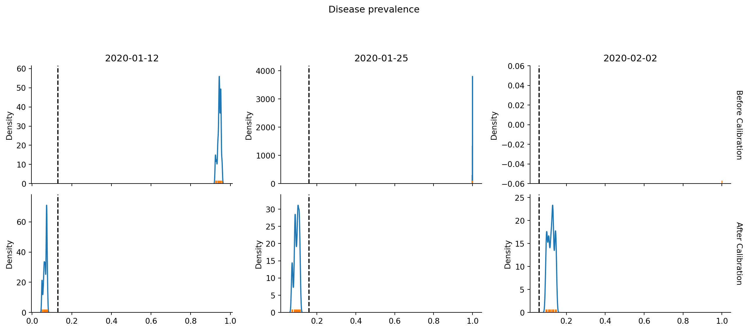

We can view some plots of the final fitted results. Whereas the two plots above were from the check_fit, running both “guess” and “best” parameters, here we make make new simulations to visualize the results.

g = calib.plot_final(); # Run the model for build_kw['n_reps'] = 15 replicates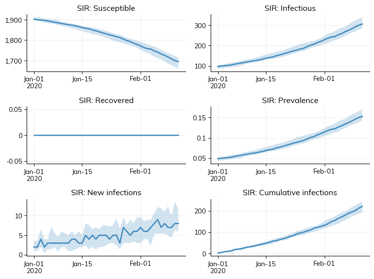

Optuna has lots of diagnostic plots that we can explore. Possible plots include:

• plot_contour
• plot_edf
• plot_hypervolume_history
• plot_intermediate_values
• plot_optimization_history
• plot_parallel_coordinate
• plot_param_importances
• plot_pareto_front
• plot_rank
• plot_slice
• plot_terminator_improvement
• plot_timeline

Here are some examples:

calib.plot_optuna('plot_optimization_history'); # Plot the optimization history

/home/runner/work/starsim/starsim/starsim/calibration.py:440: ExperimentalWarning: optuna.visualization.matplotlib._optimization_history.plot_optimization_history is experimental (supported from v2.2.0). The interface can change in the future.
  fig = getattr(vis, method)(self.study)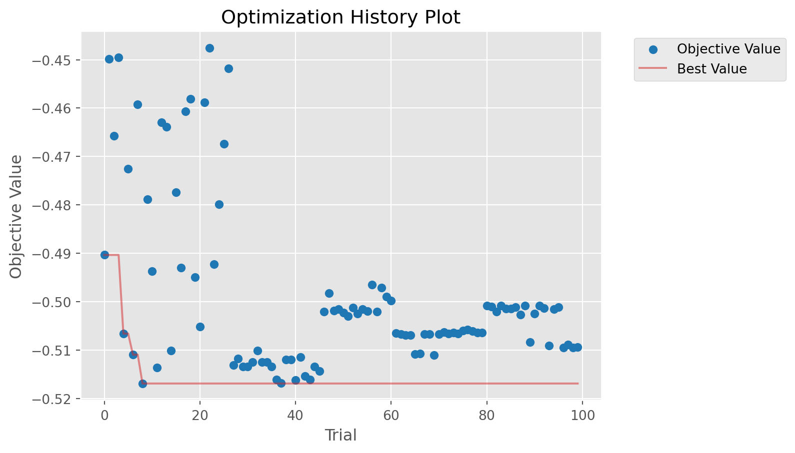

calib.plot_optuna('plot_contour');

/home/runner/work/starsim/starsim/starsim/calibration.py:438: ExperimentalWarning: optuna.visualization.matplotlib._contour.plot_contour is experimental (supported from v2.2.0). The interface can change in the future.
  fig = vis.plot_contour(self.study, params=params)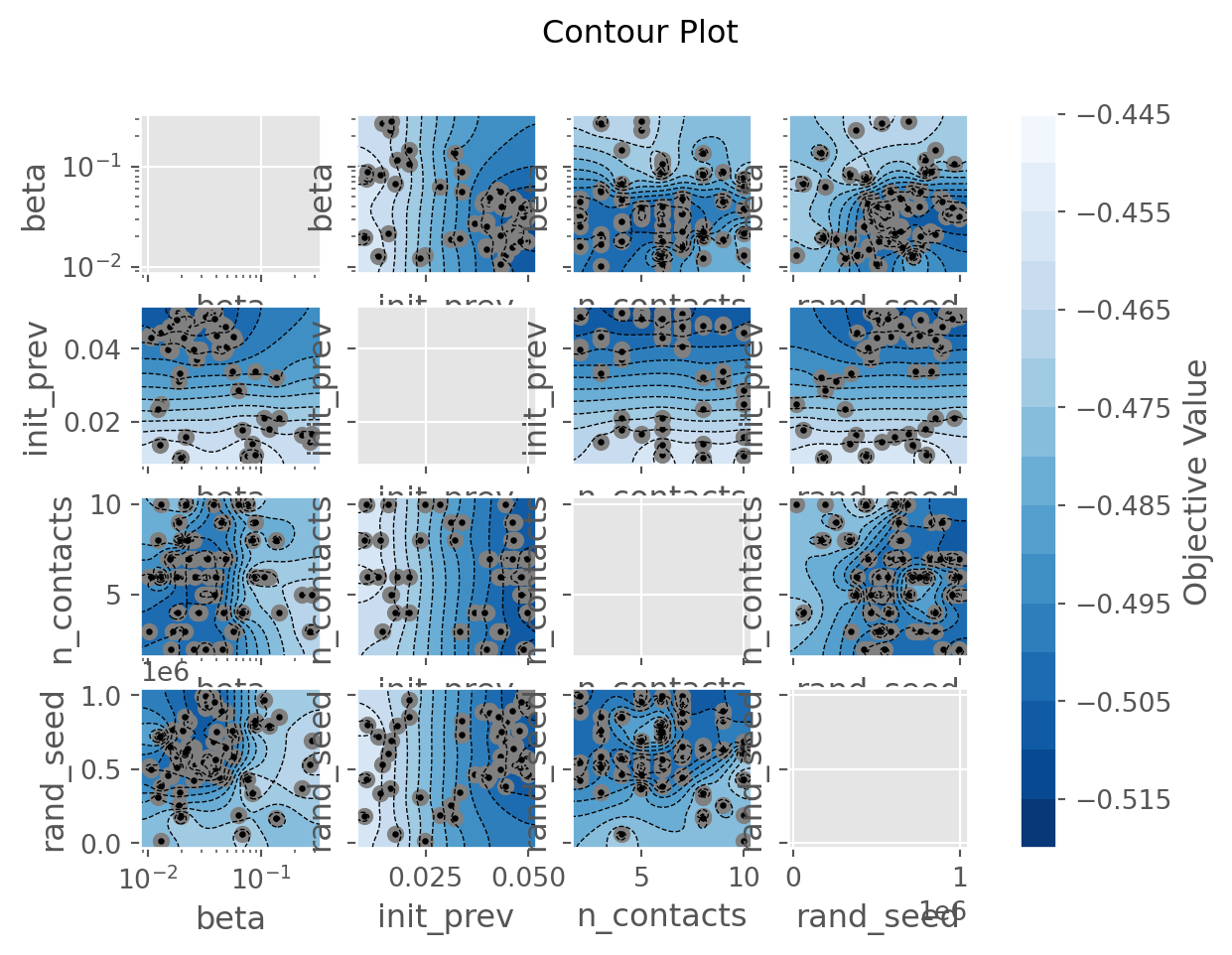

calib.plot_optuna('plot_param_importances');

Could not run plot_param_importances: Tried to import 'sklearn' but failed. Please make sure that the package is installed correctly to use this feature. Actual error: No module named 'sklearn'.

/home/runner/work/starsim/starsim/starsim/calibration.py:440: ExperimentalWarning: optuna.visualization.matplotlib._param_importances.plot_param_importances is experimental (supported from v2.2.0). The interface can change in the future.
  fig = getattr(vis, method)(self.study)

If you choose not to use components, you can always create your own mismatch function, as in the following example:

my_data = (ss.date('2020-01-12'), 0.13)

def eval(sim, expected):
    # Compute the squared error at one point in time.
    # expected will contain my_data in this example due to eval_kw
    date, p = expected
    if not isinstance(sim, ss.MultiSim):
        sim = ss.MultiSim(sims=[sim])

    ret = 0
    for s in sim.sims:
        ind = np.searchsorted(s.results.timevec, date, side='left')
        prev = s.results.sir.prevalence[ind]
        ret += (prev - p)**2
    return ret


# Define the calibration parameters
calib_pars = dict(
    beta = dict(low=0.01, high=0.30, guess=0.15, suggest_type='suggest_float', log=True),
)

# Make the sim and data
sim = make_sim()

# Make the calibration
calib = ss.Calibration(
    calib_pars = calib_pars,
    sim = sim,
    build_fn = build_sim,
    build_kw = dict(n_reps=2), # Two reps per point
    reseed = True,
    eval_fn = eval, # Will call my_function(msim, eval_kwargs)
    eval_kw = dict(expected=my_data), # Will call eval(sim, **eval_kw)
    total_trials = 20,
    n_workers = None, # None indicates to use all available CPUs
    die = True,
    debug = debug,
    verbose = 0,
)

# Perform the calibration
sc.printcyan('\nPeforming calibration...')
calib.calibrate()

# Check
calib.check_fit()

[I 2025-10-22 03:14:16,831] A new study created in RDB with name: starsim_calibration

Peforming calibration...

Fit with original pars: 1.07281525

Fit with best-fit pars: 0.0023810000000000003

✓ Calibration improved fit 1.07281525 --> 0.0023810000000000003

True

For more, take a look at test_calibration.py in the tests directory.