T2 - Building your model

The purpose of this tutorial is to introduce you to the idea of model components. In brief, these are: people, demographics, networks, diseases, interventions, analyzers, and connectors. Within Starsim, these are the ingredients of a model. On a more basic level, you can think of these as the ingredients of an epidemic. Because Starsim is intended to be very modular, you can build up all these things independently and then piece them together to make a model. Or, if that’s too complex for your needs, there are also shortcuts you can take to make life simpler!

In this tutorial we’ll focus on people, demographics, networks, diseases. The remaining components (interventions, analyzers, and connectors) will be covered later.

An interactive version of this notebook is available on Google Colab or Binder.

Simple SIR model

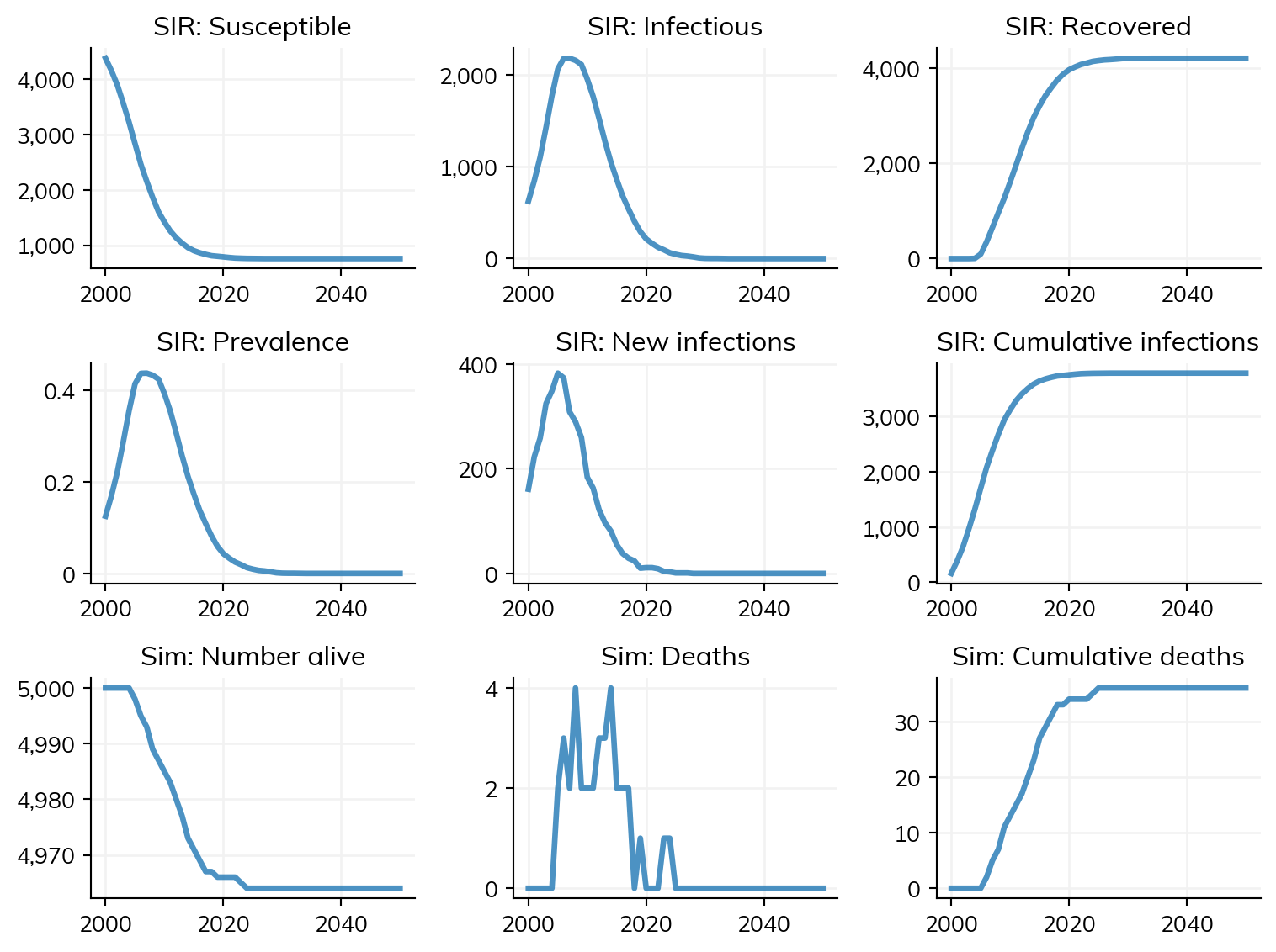
Let’s revisit the simple SIR model from Tutorial 1:

import starsim as ss

# Define the parameters
pars = dict(
    n_agents = 5_000,     # Number of agents to simulate
    networks = dict(      # *Networks* add detail on how the agents interact with each other 
        type = 'random',  # Here, we use a 'random' network
        n_contacts = 4    # Each person has an average of 4 contacts with other people
    ),
    diseases = dict(      # *Diseases* add detail on what diseases to model 
        type = 'sir',     # Here, we're creating an SIR disease 
        init_prev = 0.1,  # Proportion of the population initially infected 
        beta = 0.1,       # Probability of transmission between contacts
    )
)

# Make the sim, run and plot
sim = ss.Sim(pars)
sim.run()
sim.plot()

Initializing sim with 5000 agents
  Running 2000.01.01 ( 0/51) (0.00 s)  ———————————————————— 2%
  Running 2010.01.01 (10/51) (0.15 s)  ••••———————————————— 22%
  Running 2020.01.01 (20/51) (0.18 s)  ••••••••———————————— 41%
  Running 2030.01.01 (30/51) (0.20 s)  ••••••••••••———————— 61%
  Running 2040.01.01 (40/51) (0.21 s)  ••••••••••••••••———— 80%
  Running 2050.01.01 (50/51) (0.23 s)  •••••••••••••••••••• 100%

Figure(768x576)

Now let’s look at the pars dictionary in more detail. The one we’ve created here has 3 things in it: the number of agents (n_agents), detail on how the agents interact with each other (networks) and detail on what disease we’re modeling (diseases). When we create and run the model, what happens ‘under the hood’ is that the simulation creates 5,000 people, and allows them to the interact with one another over the network and transmit the infection.

Simple SIR model built with components

The example above is a nice simple way to get started, but you might want to have more control over the networks, diseases, and people that you’re creating. Here’s another version of the exact same model, but written slightly differently:

people = ss.People(n_agents=5_000)
network = ss.RandomNet(n_contacts=4)
sir = ss.SIR(init_prev=0.1, beta=0.1)
sim = ss.Sim(diseases=sir, people=people, networks=network)
sim.run()
sim.plot()

Initializing sim with 5000 agents
  Running 2000.01.01 ( 0/51) (0.00 s)  ———————————————————— 2%
  Running 2010.01.01 (10/51) (0.02 s)  ••••———————————————— 22%
  Running 2020.01.01 (20/51) (0.04 s)  ••••••••———————————— 41%
  Running 2030.01.01 (30/51) (0.06 s)  ••••••••••••———————— 61%
  Running 2040.01.01 (40/51) (0.08 s)  ••••••••••••••••———— 80%
  Running 2050.01.01 (50/51) (0.09 s)  •••••••••••••••••••• 100%

Figure(768x576)

Rather than bundling everything under pars, we’re now defining components individually for people, networks, and diseases. As for the disease/network details, instead of putting all information in one bucket (pars['diseases'] = dict(name='sir', init_prev=0.1, beta=0.1)), we’re now using ss.SIR()which serves as a prepared ‘template’ where we fill in the details. This new way provides us more flexibility to adjust details of the disease as we need.

Don’t worry if you have not seen or used these ‘templates’ (called custom classes in programming) before, but imagine them as special containers that come with predefined tools (aka built-in methods) to streamline your modelling process. Even if you’re not an expert programmer, these ‘templates’ are intuitive to use and they will serve as our go-to solution as we move through the examples.

Now, let’s look at a few useful ways to improve our model by extending these three components (people, networks, and diseases).

Making changes to our components

One of the main advantages of agent-based models is they allow you to capture heterogeneity between people. In real life, it’s not realistic that everyone in a population has the same number of contacts with other people. Let’s make our contact network more realistic by adding some variation here. For this, we’ll use a Poisson distribution. The two lines below both do the same thing:

network = ss.RandomNet(n_contacts= ss.poisson(4))
network = ss.RandomNet(n_contacts=dict(type='poisson', lam=4))

If we use this network, our agents will have varying numbers of contacts.

Accessing results

Once you’ve run a model, you will want to see what the results look like! We’ve seen a few basic plotting commands above, but if you want to inspect the results for yourself, you can take a look in sim.results. This is a dictionary with keys corresponding to core components of interest. For example, the sim we created in the code block above will have the following keys: ['n_alive', 'new_deaths', 'births', 'deaths', 'sir']. Then sim.results.sir is also a dictionary and contains all the results relating to this disease over time. For example, new_infections is a kind of array showing annual new infections.

Matters of time

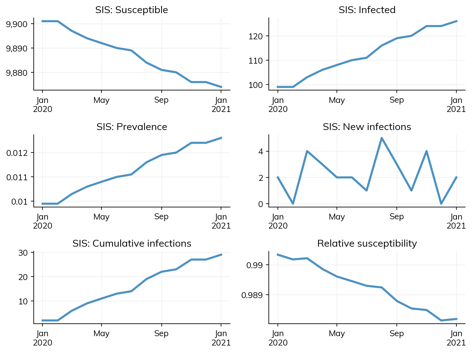
The default for Starsim models is the start simulations in 1995 and simulate with an annual timestep for 35 years. All of this can be easily changed within the main pars dictionary or by passing alternative values straight to the sim, e.g.

sim = ss.Sim(start='2020-01-01', stop='2021-01-01', dt=ss.months(1), diseases='sis', networks=network)  # Simulate from 2020 for 1 year with a monthly timestep
sim.run().plot()

Initializing sim with 10000 agents
  Running 2020.01.01 ( 0/13) (0.00 s)  •——————————————————— 8%
  Running 2020.11.01 (10/13) (0.02 s)  ••••••••••••••••———— 85%
Figure(768x576)

Loading and saving

You can save a sim to disk with sim.save(), and then reload it:

sim.save('example.sim')
new_sim = ss.load('example.sim')

By default, to save space, this saves a “shrunken” version of the sim with most of the large objects (e.g. the People) removed. To save everything (for example, if you want to save a partially run sim, then reload it and continue running), you can use shrink=False:

sim.save('example-big.sim', shrink=False)

'/home/cliffk/idm/starsim/docs/tutorials/example-big.sim'

All Starsim objects can also be saved via ss.save(); this will save the entire object. This is useful for quickly storing objects for use by other Python functions, for example:

df = sim.to_df()
ss.save('example.df', df)
new_df = ss.load('example.df')

However, for a human-readable format, you may want to use a different format. For example, if you’ve exported the results as a dataframe, you can then save as an Excel file:

df.to_excel('example.xlsx')

Summary

You’ve now seen how to create models using the “sim” class (ss.Sim), either by defining a dictionary of parameters or by passing in sim components (demographics, people, diseases, and networks). This means you’ve got the basic skills needed to start making models to answer a range of different questions. We’ll close this tutorial with a few examples that you might like to try out for yourself.

Exercises

How would you model an outbreak of an SIR-like disease within a refugee camp of 20,000 people? Suppose you were interested in the cumulative number of people who got infected over 1 year - how would you find this out?
Whether an epidemic ‘takes off’ depends to a large extent on the basic reproduction number, which is the expected number of cases that an infected individual generates. In an agent based model like the one we’ve created here, that depends largely on three things: beta (the transmissibility parameter for the disease), n_contacts (the number of contacts each person has), and dur_inf (another disease-related parameter that determines the duration of infection). Experiment with different values for each of these and compare the trajectory of sim.results.sir.n_infected with different parameter values.