Agent-based models draw random numbers from distributions to simulate various phenomena. Realizations (also called draws or samples) from distributions are used to model everything from the duration of each infection to the number of contacts each individual has in a network to the outcomes of individual diagnostic tests. The Starsim framework includes state of the art functionality for specifying and sampling from statistical distributions.
In this guide, you will:
Learn which distributions are available in Starsim.
See how to use Starsim framework functionality to create a frozen distribution, generate samples, visualize the distribution, and extract statistics.
Set or update model parameters that are distributions.
Use distributions with “dynamic parameters” that depend on agent attributes, the simulation time, or other factors.
Build an example Starsim intervention that uses a distribution with dynamic parameters.
One key advantage of Starsim distributions is that they enable low-variance comparison between simulations through a technique called “common random numbers” (CRN). To learn more about CRN, see the Common Random Numbers guide.
Available distributions
The starsim framework includes a wide range of distributions that can be used to model various phenomena. The following distributions are available:
Distribution
Starsim Dist
Parameters
Description
Random
random
None
Random number between 0 and 1.
Uniform
uniform
low, high
Random number between a specified minimum and maximum.
Normal
normal
loc (mean), scale (standard deviation)
Random number from a normal (Gaussian) distribution with specified mean and standard deviation.
Lognormal (implicit)
lognormal_im
mean, sigma (of the underlying normal distribution)
Random number from a lognormal distribution specified by the mean and standard deviation of the underlying normal distribution.
Lognormal (explicit)
lognormal_ex
mean, std (of the distribution itself; mean must be positive)
Random number from a lognormal distribution specified by the mean and standard deviation of the distribution itself.
Exponential
expon
scale (mean of the distribution, equivalent to 1/λ)
Random number from an exponential distribution with specified scale parameter.
Poisson
poisson
lam
Random number from a Poisson distribution with specified rate parameter.
Negative Binomial
nbinom
n, p (number of successes, probability of success)
Random number from a negative binomial distribution with specified parameters.
Weibull
weibull
c (shape parameter, sometimes called “k”), loc (shifts the distribution), scale (sometimes called “λ”)
Random number from a Weibull distribution with specified parameters, uses scipy’s weibull_min.
Gamma
gamma
a (shape parameter, sometimes called “k”), loc (shifts the distribution), scale (sometimes called “θ”)
Random number from a gamma distribution with specified shape and scale parameters.
Beta
beta_dist
a (shape parameter, must be > 0), b (shape parameter, must be > 0)
Random number from a beta distribution with specified shape parameters.
Constant
constant
v
Constant value, useful for fixed parameters and testing.
Random Integer
randint
low, high
Random integer between a specified minimum and maximum.
Bernoulli
bernoulli
p
Random number from a Bernoulli distribution with specified probability of success. Bernoulli distributions are used frequently to determine binary outcomes, such as whether an agent is infected or not.
Choice
choice
a (int or list of choices), p (probability of each choice)
Randomly select from a list of values. This distribution only supports fixed parameters.
Histogram
histogram
values, bins, density, data
Random number from a histogram distribution specified by a list of values and their corresponding probabilities.
You can also create a custom distribution by extending the Dist class from Starsim.
How to use Starsim distributions
Parameters for Starsim distributions can have fixed parameters (the same for all agents) or vary dynamically. We will start with a simple normal distribution with fixed parameters:
import starsim as ssss.options(jupyter=True)import numpy as np# Create a Normal distribution with mean 0 and standard deviation 1# The "strict" flag is needed only for this example to avoid warningsd = ss.normal(name="Normal with fixed parameters", loc=0, scale=1, strict=False)# ^^^ The above "d" object is the "frozen" distribution.print(d)
ss.normal(loc=0, scale=1)
Drawing samples
Samples from a distribution can be drawn using the rvs method.
While possible to request a specific number of samples, as shown below, please know that this is not the preferred way to use distribution in Starsim:
The above approach is better than calling numpy.random directly, but still not ideal because it does not allow for dynamic parameter nor low-noise sampling. Therefore, please instead call the rvs method with the unique identifiers (uids) of the agents for which you need samples. Alternatively, you can pass a boolean mask of length equal to the number of agents in the simulation:
# Create a simulation for context# [you will not need to do this when working within the framework]sim = ss.Sim(n_agents=10).init()# Specify the distribution, here a random integer between -10 and 10d_sim = ss.randint(name="Random integer with fixed parameters", low=-10, high=10)d_sim.init(sim=sim) # Initialize the distribution [done automatically in the framework]# Instead of requesting 5 random numbers, the preferred pattern is to request# random numbers for specific agents by passing a list of agent IDs. Doing so# enable the powerful dynamic parameters to be used while also supporting the# low-noise common random number sampling.draws = d_sim.rvs([3, 5, 2, 9, 4]) # Draw samples for specific agents by UIDprint(f"Draws for agents 3, 5, 2, 9, and 4: {draws}")mask = sim.people.age <25draws_mask = d_sim.rvs(mask) # Draw samples for agents under 25 from a boolean maskprint(f"Draws for agents under 25: {draws_mask}")draws_all = d_sim.rvs(sim.people.uid) # Draw samples for all agentsprint(f"Draws for all agents (0, 1, 2, ..., n_agents): {draws_all}")
Initializing sim with 10 agents
Draws for agents 3, 5, 2, 9, and 4: [ 0  0  9  5 -4]
Draws for agents under 25: [-5  2 -6 -6 -2]
Draws for all agents (0, 1, 2, ..., n_agents): [ 8  7  0  0  0  6 -6 -6  1 -7]
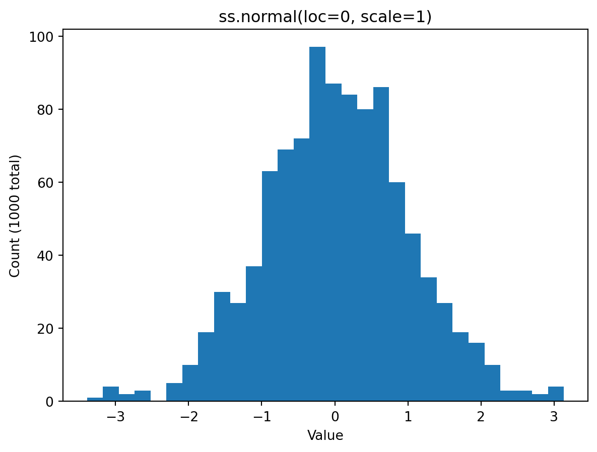
Visualizing distributions
Let’s take a look at the distribution by plotting a histogram of samples:
rvs = d.plot_hist(n=1000, bins=30)
Extracting distribution statistics
We can quickly calculate statistics of the distribution by accessing the underlying “dist” property of the distribution:
Mean: 0.0
Standard Deviation: 1.0
95% Interval: [-1.95996398  1.95996398]
Setting model parameters that are distributions
Many Starsim modules directly expose distributions as parameters for user customization. For example, the SIR disease module has three parameters are distributions:
Parameter
Meaning
Default Value
init_prev
Initial prevalence of infection
ss.bernoulli(p=0.01)
dur_inf
Duration of infection
ss.lognorm_ex(mean=ss.dur(6))
p_death
Probability of death given infection
ss.bernoulli(p=0.01)
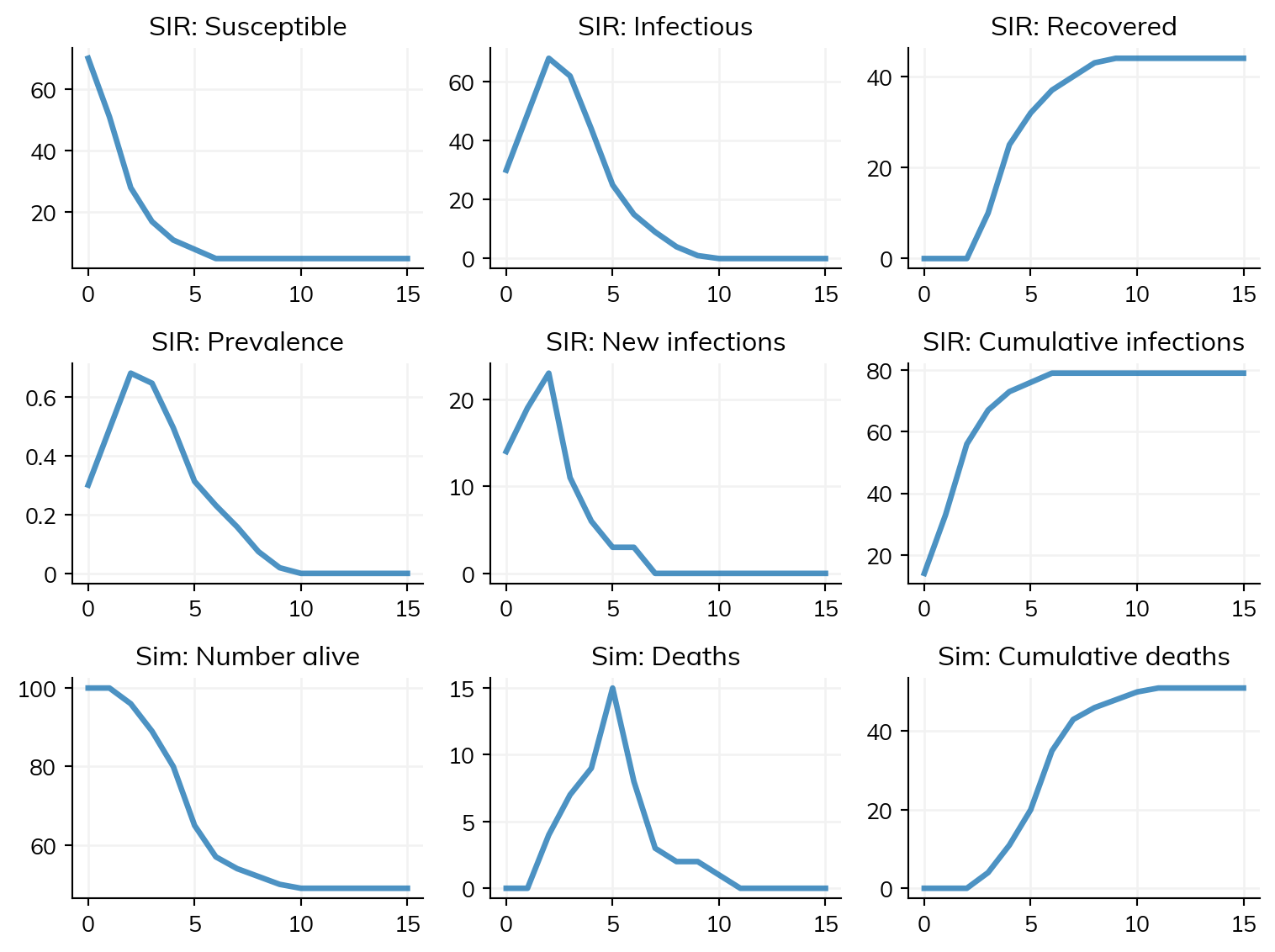
You can change these parameters away from their defaults by passing in a different distribution, as demonstrated below:
sir = ss.SIR(# Set the init_prev parameter to randomly infect 15% of the population init_prev = ss.bernoulli(p=0.15),# Set the dur_inf parameter to a Weibull dur_inf = ss.weibull(c=2, loc=1, scale=2))# Alternatively, update parameters of a default distributionsir.pars.p_death.set(p=0.5) # Update the death probability to 50%# Create, run, and plot a sim using the SIR disease modelsim = ss.Sim(n_agents=100, diseases=sir, dur=15, dt=1, start=0, networks=ss.RandomNet())sim.run().plot()
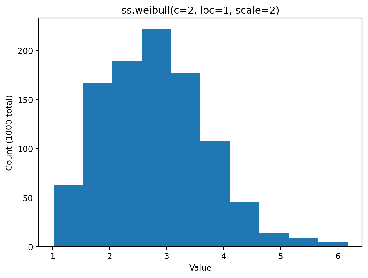
It’s easy to inspect distributions, for example dur_inf of the SIR module using plot_hist.
NOTE: in the code below that we access dur_inf at sim.diseases.sir.pars rather than at sir.pars (referencing the module in the previous cell) because Starsim makes a copy. The sir is not initialized and does not have the sim context.
rvs = sim.diseases.sir.pars.dur_inf.plot_hist()
Using distributions with dynamic parameters
Up to this point, the distributions we have used have had fixed parameters. Every agent draws will draw from the same distribution at every time step. But Starsim has a powerful feature to specify distributions with dynamic parameters that can change based on agent attributes, simulation time, or other factors.
Let’s continue with the SIR example, but make the initial prevalence of infection depend on the age of the agent. Instead of a fixed probability for all agents, let’s make it so that children under 15 years old have a 25% chance of being selected as a “seed” infection and adults over 15 years old have a 10% chance.
To implement dynamic parameters, we set the parameter (p in the case of a Bernoulli distribution) to a callable like a function. The callable must accept three arguments:
uids: The unique IDs of the agents being processed
It should return a numpy array of the same length as uids containing the parameter value for each agent, or a scalar if the parameter is the same for all agents.
def set_p_by_age(self, sim, uids): p = np.full(len(uids), fill_value=0.10) # Default 10% infection probability p[sim.people.age <15] =0.25# 25% for ages < 15# For demonstration, print the age and probability for each agent:for uid, age, prob inzip(uids, sim.people.age[uids], p):print(f"Agent {uid} | Age: {age:5.2f} | Infection Seed Probability: {prob:.0%}")return psir = ss.SIR(# Set init_prev as a dynamic parameter init_prev = ss.bernoulli(p=set_p_by_age),)# Create, run, and plot a sim using the SIR disease modelsim = ss.Sim(n_agents=10, diseases=[sir], dur=30)sim.run()
Example Starsim intervention using dynamic distributions
To demonstrate the use and power of distributions in the Starsim framework, we next create an intervention that delivers a vaccine to a random subset of agents using a Bernoulli distribution. The default distribution will be fixed, the same for all agents, but we’ll make it a parameter to that the user can change it without having to modify the source code.
NOTE: That we create the distribution only one time in the __init__ method of the intervention. Here, the distribution is part of the parameters, so will appear at self.pars.p_vx. Alternatively, we could create a distribution between update_pars and return, as noted. Please avoid recreating a Starsim distribution on every time step.
class MyVx(ss.Intervention):def__init__(self, pars=None, **kwargs):super().__init__()self.define_states( ss.BoolState('vaccinated', label="Vaccinated", default=False) )self.define_pars(# Create a Bernoulli distribution as a module parameter# The value p=0.1 is a placeholder, the user will override p_vx = ss.bernoulli(p=0.1, name="Vaccination Probability") )self.update_pars(pars=pars, **kwargs)# NOTE, this is a great place to create other distributions, for example# self.my_dist = ss.normal(loc=0, scale=1)returndef init_results(self):super().init_results()self.define_results( ss.Result('new_vx', dtype=int, label="Newly Vaccinated") )returndef step(self):# Choose which agents to vaccinate novx =self.vaccinated ==False# Boolean mask# Filter to select agents for which the Bernoulli sample is True vx_uids =self.pars.p_vx.filter(novx) # <-- can pass in mask or uidsself.vaccinated[vx_uids] =True# Set the state to vaccinated sim.diseases.sir.rel_sus[vx_uids] =0.0# Set susceptibility to 0 for vaccinated agents# Store the resultsself.results.new_vx[sim.ti] =len(vx_uids)
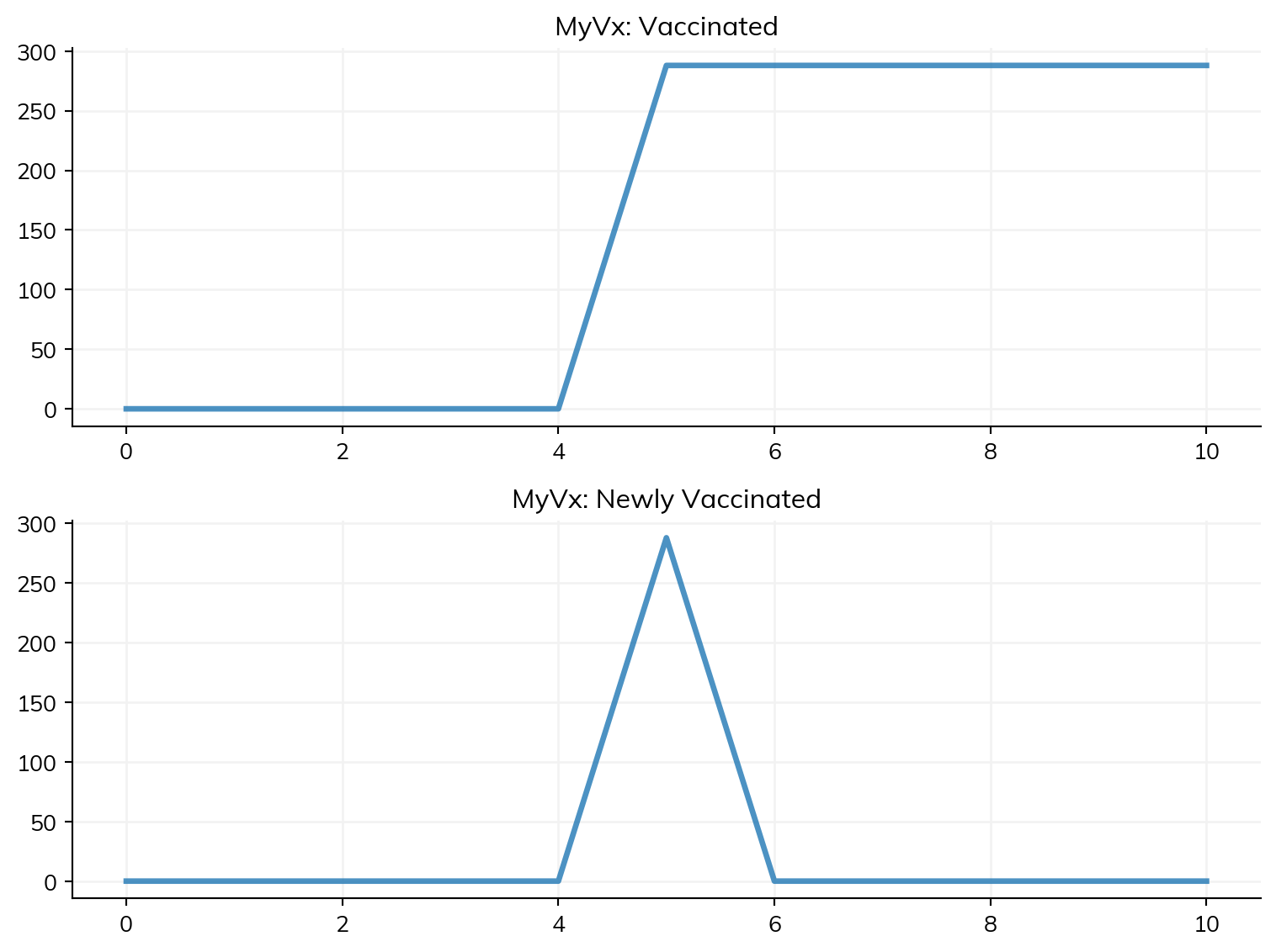
Now that we have created the intervention, we can configure it with a custom p_vx_func in “user space” and run the simulation.
def p_vx_func(self, sim, uids):# Set the probability of vaccination for each agent in uids# This is the "dynamic" callable for p_vx# Let's only administer the vaccine on the 5th time stepif sim.ti !=5:return0.0# Set vaccination probability proportional to age p = sim.people.age[uids] /100.0# Normalize age to a probability between 0 and 1 p = p.clip(0.0, 1.0) # Ensure probabilities are between 0 and 1return p # p has the same length as uidsvx_intv = MyVx(p_vx = ss.bernoulli(p=p_vx_func))# Create, run, and plot a sim using the SIR disease modelsim = ss.Sim(n_agents=1000, dur=10, dt=1, start=0, diseases=ss.SIR(), # Default SIR disease model interventions=[vx_intv], networks=ss.RandomNet())sim.run().plot('myvx') # Verify vaccinations only on the 5th time step
See how vaccines were delivered only on time step 5? If we were to look at which agents received the vaccine, we would see probability increasing with age.