These are the solutions to the exercises from each of the tutorials. Many of these exercises are open-ended, so these are just example solutions — there are often many equally valid approaches. If you get stuck or want to discuss alternatives, email us!
An interactive version of this notebook is available on Google Colab or Binder.
Let’s start with the simplest version of a Starsim model. We’ll make a version of a classic SIR model. Here’s how our code would look:
T1 Solutions
Question 1
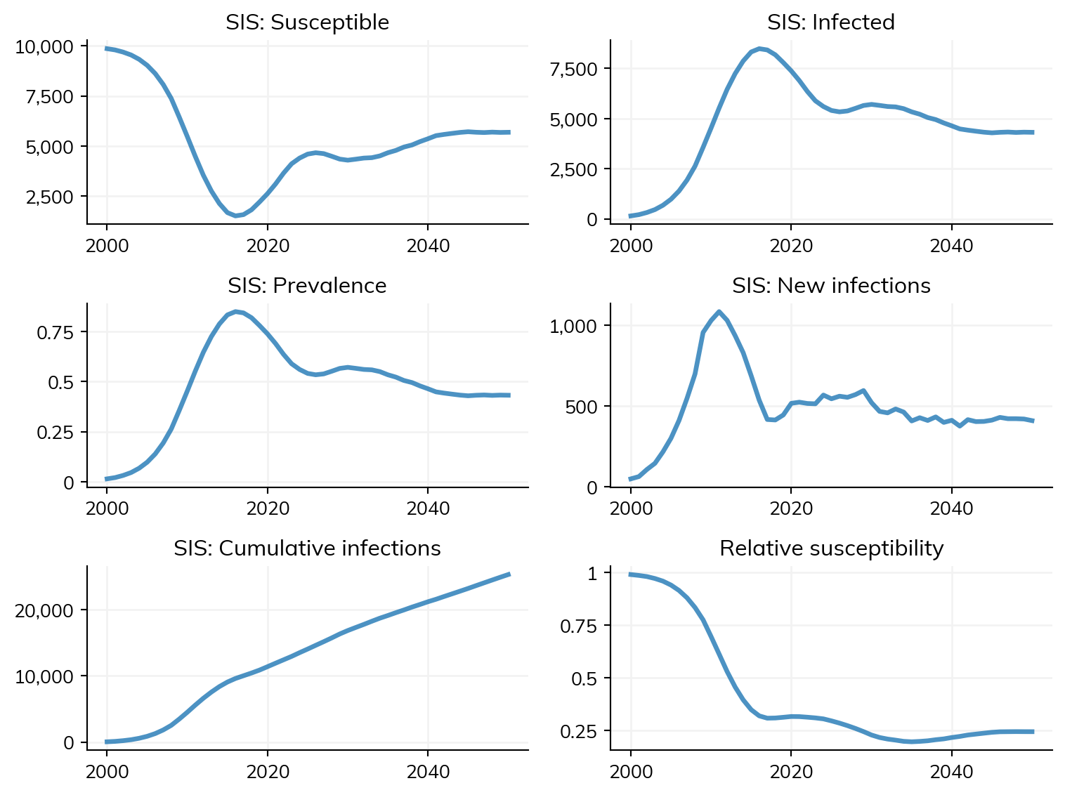
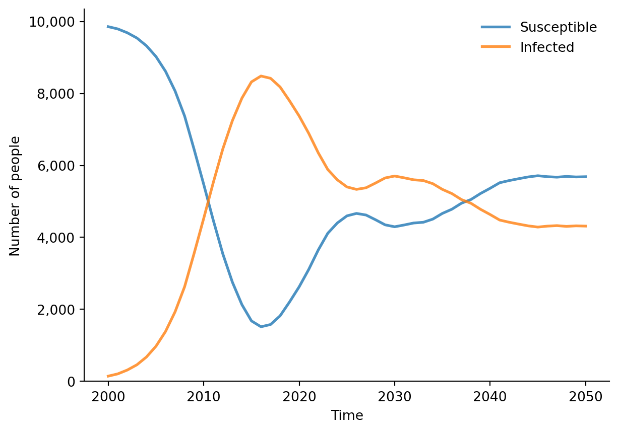
Q: To simulate a susceptible-infectious-susceptible (SIS) model instead of SIR, what would we change in the example above?
A: We would simply change 'sir' to 'sis':
import starsim as ssss.options(jupyter=True)import sciris as sc# Define the parameterspars = sc.objdict( # We use objdict to allow "." access n_agents =10_000, networks = sc.objdict(type='random', n_contacts =10, ), diseases = sc.objdict(type='sis', # <-- change this init_prev =0.01, beta =0.05, ))# Make the sim, run and plotsim = ss.Sim(pars)sim.run()sim.plot()sim.diseases.sis.plot() # <-- change this
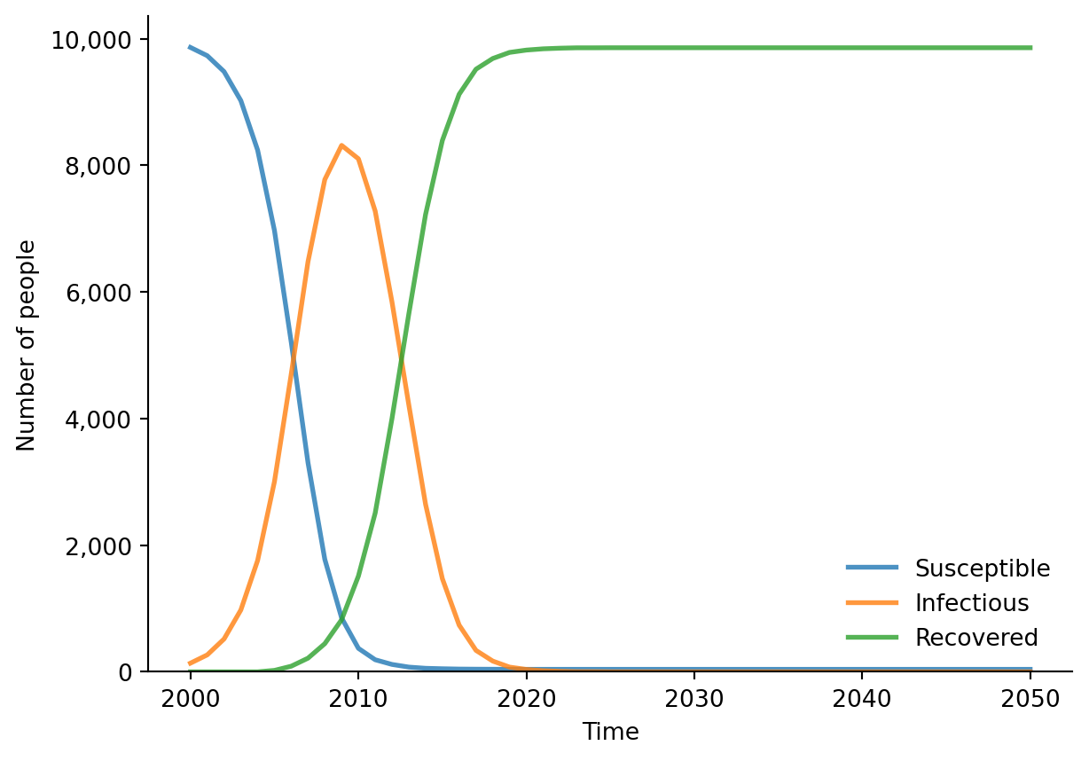
Q: How do the results change if we increase/decrease beta?
Increasing beta makes the curves steeper:
pars.diseases.type='sir'# Switch back to SIRpars2 = sc.dcp(pars) # copy to new dictionarypars2.diseases.beta =0.10sim2 = ss.Sim(pars2).run()sim2.diseases.sir.plot()
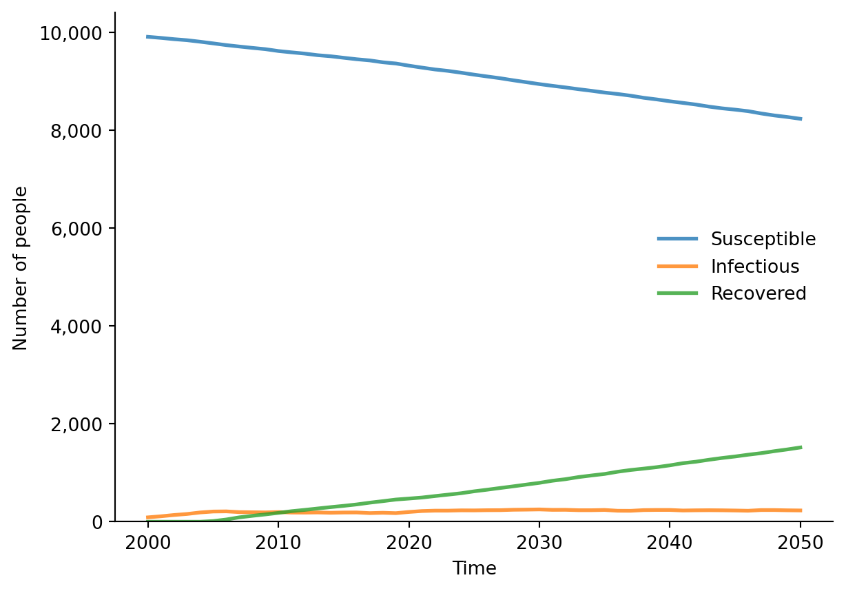
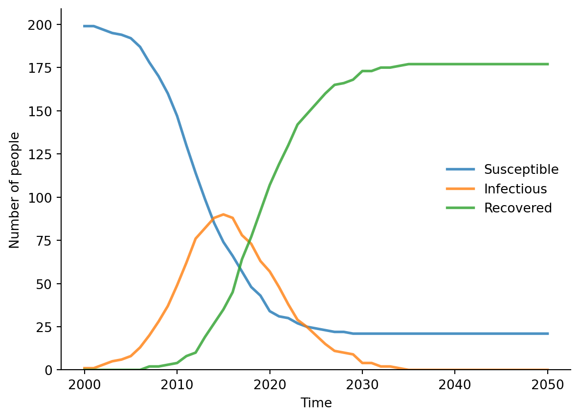
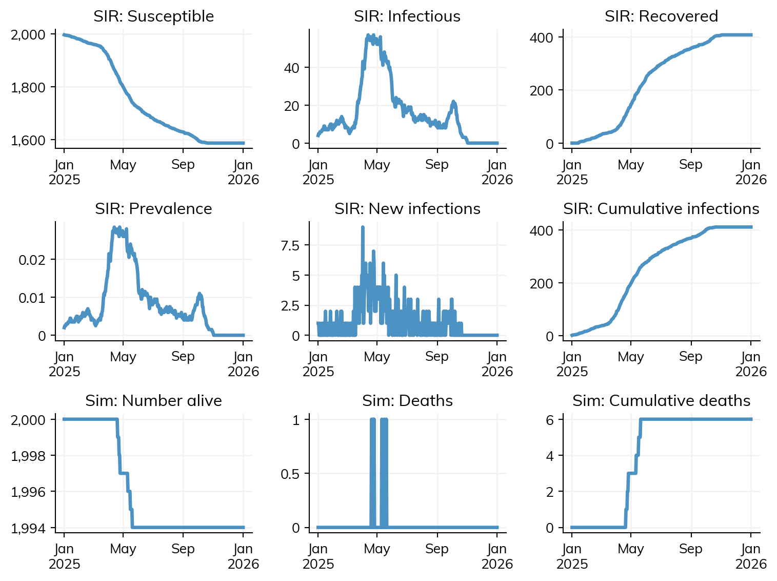
Q: How would you model an outbreak of an SIR-like disease within a refugee camp of 2,000 people? Suppose you were interested in the cumulative number of people who got infected over 1 year - how would you find this out?
The answer obviously depends on the disease parameters. However, we can make some simple assumptions and use cum_infections to determine the total number of infections:
import starsim as ssimport sciris as scpars = sc.objdict( n_agents =2_000, start ='2025-01-01', dur =365, dt ='day', verbose =1/30, # Print every month)sir = ss.SIR( dur_inf = ss.days(14), beta = ss.perday(0.02), init_prev =0.001,)net = ss.RandomNet(n_contacts=4)sim = ss.Sim(pars, diseases=sir, networks=net)sim.init()sim.run()sim.plot()answer = sim.results.sir.cum_infections[-1]print(f'Cumulative infections over one year: {answer}')
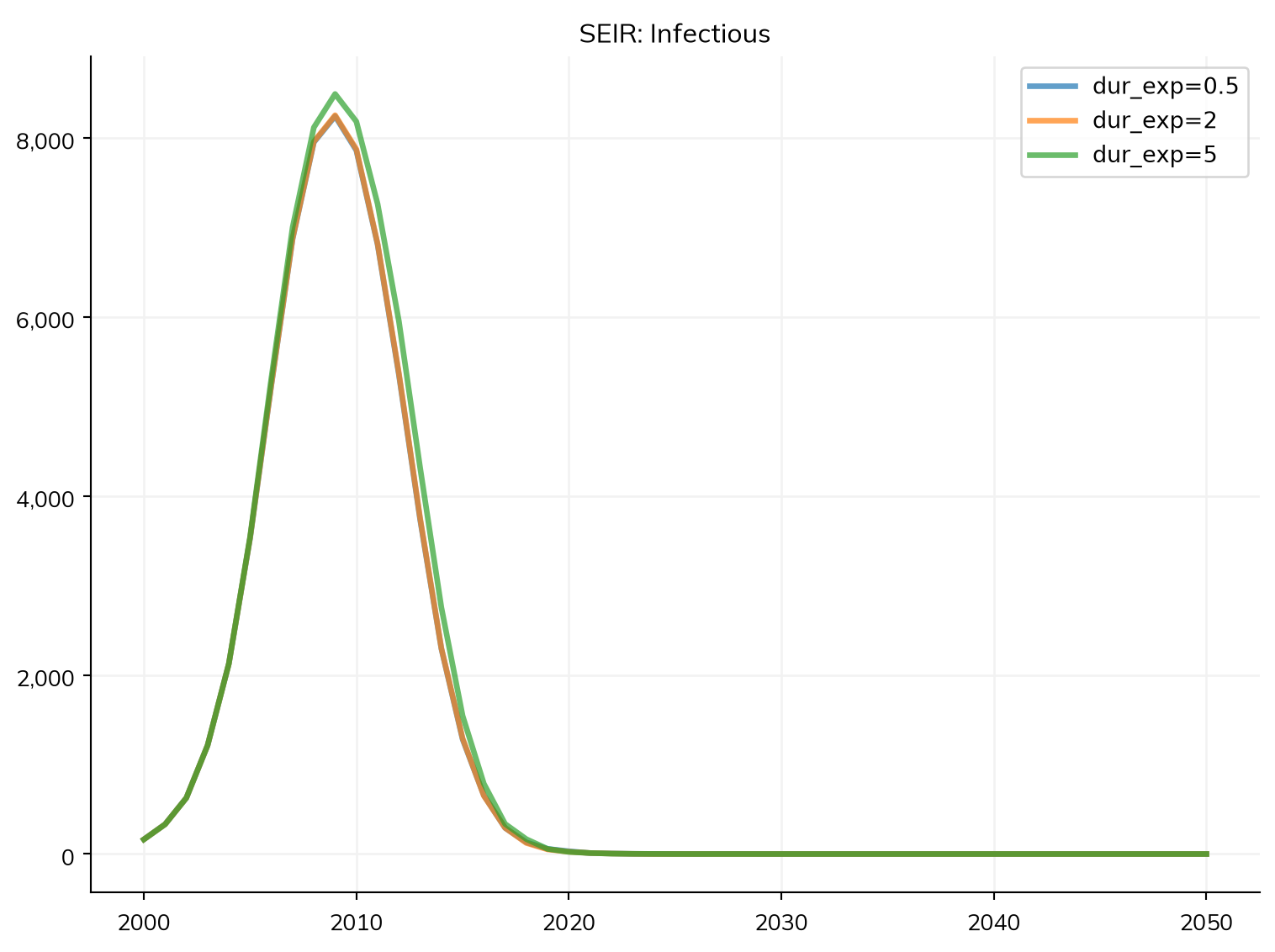
Q: Whether an epidemic ‘takes off’ depends to a large extent on the basic reproduction number, which in this kind of model depends on beta, n_contacts, and dur_inf. Experiment with different values for each and compare the trajectory of sim.results.sir.n_infected.
A: All three parameters increase transmission, so increasing any of them makes the epidemic grow faster and larger. The cleanest way to see this is to write a small helper that builds a sim for a given set of parameters, then compare them:
import starsim as ssimport sciris as scdef make_sim(beta=0.05, n_contacts=10, dur_inf=10): pars = sc.objdict( n_agents =5_000, networks = sc.objdict(type='random', n_contacts=n_contacts), diseases = sc.objdict(type='sir', init_prev=0.01, beta=beta, dur_inf=dur_inf), verbose =0, )return ss.Sim(pars, label=f'beta={beta}, n_contacts={n_contacts}, dur_inf={dur_inf}')# Vary each parameter in turn, relative to the baselinesims = [ make_sim(), # Baseline make_sim(beta=0.10), # Higher transmissibility make_sim(n_contacts=20), # More contacts make_sim(dur_inf=20), # Longer infectious period]msim = ss.parallel(sims)msim.plot('sir_n_infected')
Figure(768x576)
Each of the three modified scenarios produces a larger, faster epidemic than the baseline, illustrating that they all push the reproduction number in the same direction.
T3 Solutions
Question 1
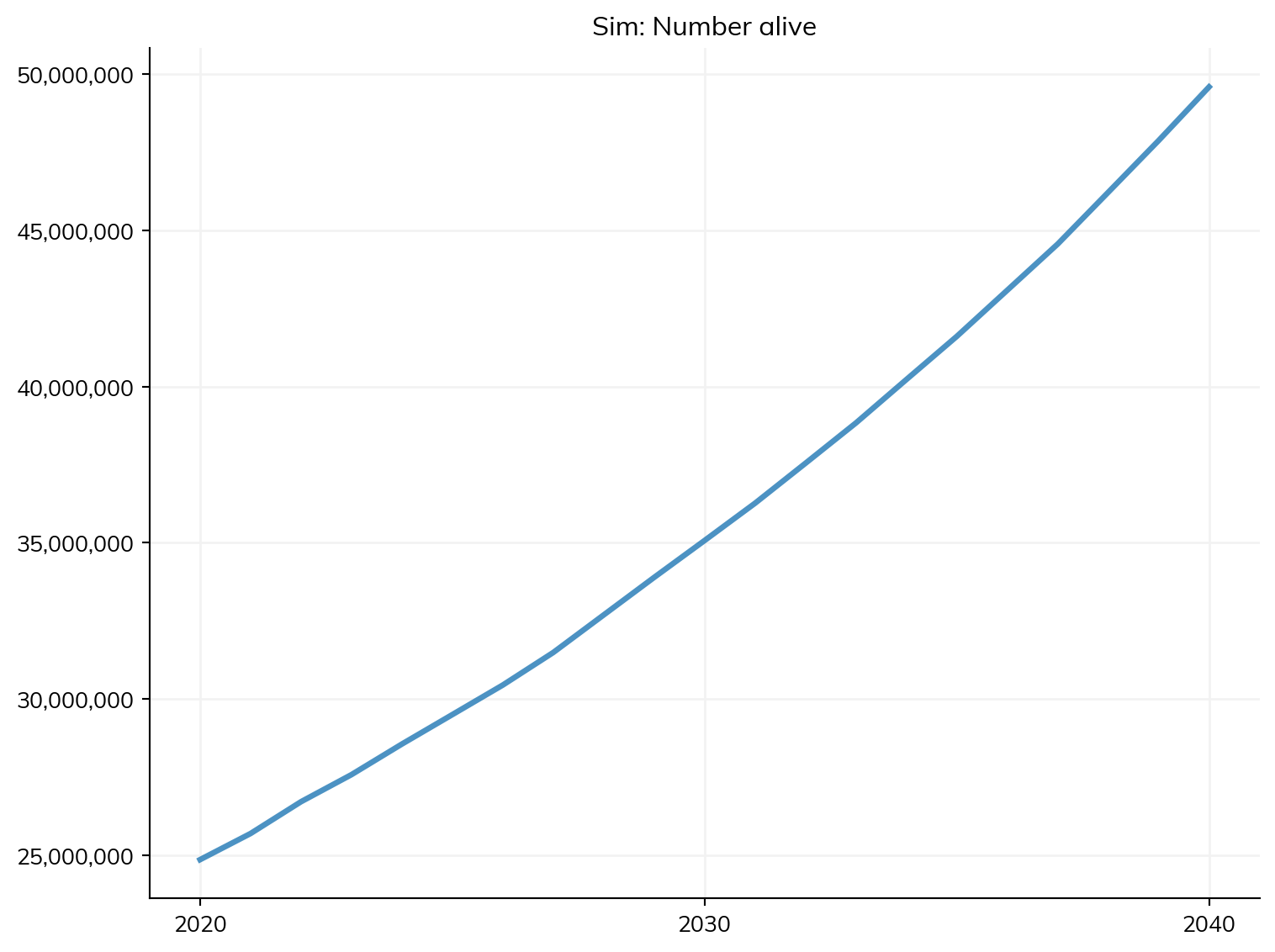
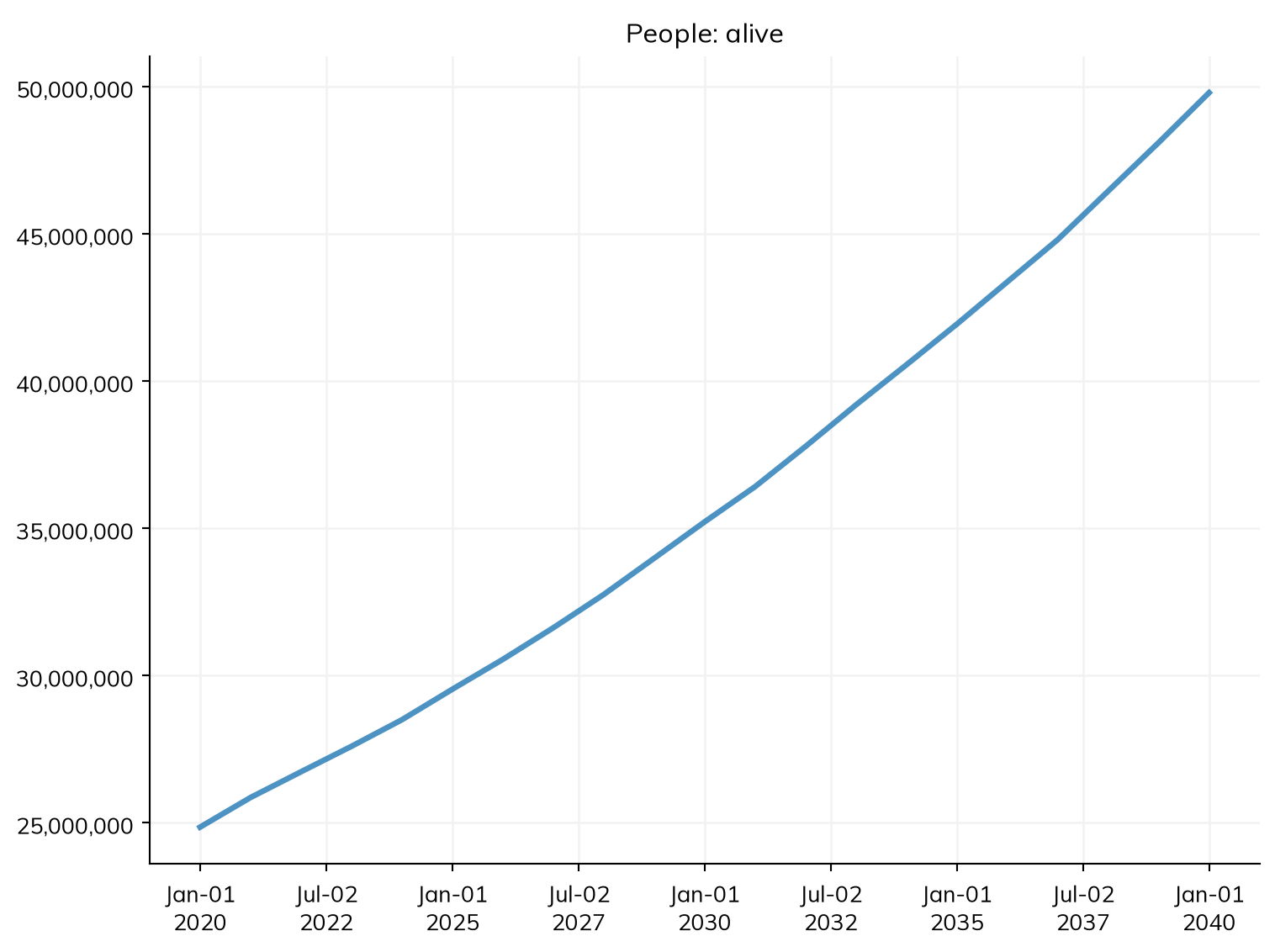
Q: In Niger, the crude birth rate is 45 and the crude death rate is 9. Assuming these rates stay constant, and starting with a total population of 24 million in 2020, how many people will there be in 2040? (You do not need to include any diseases in your model.)
A: We can build our simple demographic model with these parameters, then run it and plot the results:
import starsim as ssimport sciris as scpars = sc.objdict( start =2020, stop =2040, total_pop =24e6, birth_rate =45, death_rate =9,)sim = ss.Sim(pars)sim.run()sim.plot('n_alive')answer = sim.results.n_alive[-1]/1e6print(f'Population size in year {pars.stop}: {answer} million')
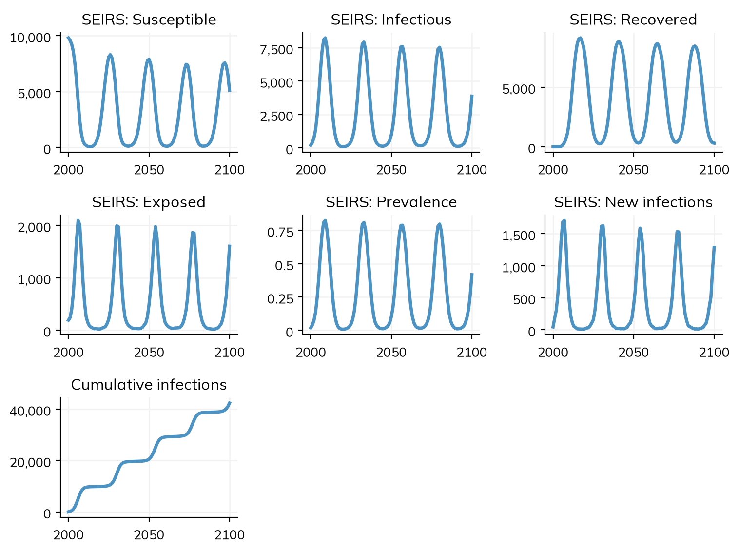
Q: Adapt the SEIR example to be SEIRS (where recovered people can become susceptible again).
A: We add a duration of immunity (dur_imm) and, in step_state(), move recovered agents back to susceptible once their immunity has waned. We schedule the waning time in set_prognoses() for everyone who is going to recover:
class SEIRS(SEIR):def__init__(self, pars=None, *args, **kwargs):super().__init__()self.define_pars(dur_imm=ss.lognorm_ex(10)) # Duration of immunity after recoveryself.update_pars(pars, **kwargs)self.define_states(ss.FloatArr('ti_susceptible'))returndef step_state(self):super().step_state()# Recovered agents whose immunity has waned return to susceptible waning =self.recovered & (self.ti_susceptible <=self.ti)self.recovered[waning] =Falseself.susceptible[waning] =Truereturndef set_prognoses(self, uids, sources=None):super().set_prognoses(uids, sources)# Schedule waning of immunity for those who will recover recovering = uids[~np.isnan(self.ti_recovered[uids])] dur_imm =self.pars.dur_imm.rvs(recovering)self.ti_susceptible[recovering] =self.ti_recovered[recovering] + dur_immreturnseirs = SEIRS()sim = ss.Sim(diseases=seirs, networks='random', dur=100, verbose=0)sim.run()sim.plot('seirs')
Figure(768x576)
Unlike the SEIR model, the SEIRS model can sustain endemic transmission, because the pool of susceptibles is continually replenished as immunity wanes.
Question 3
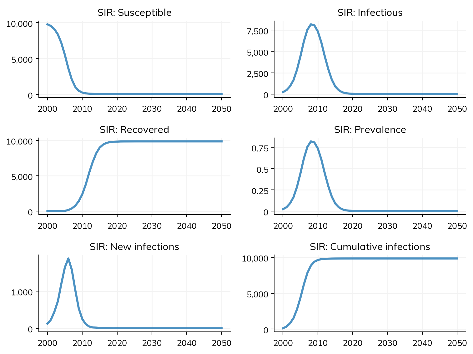
Q: Can you create a model with two strains of the same disease that provide partial cross-immunity?
A: One clean way to do this is to model the two strains as two separate diseases, and use a connector to couple them: recovery from one strain reduces susceptibility to the other. Here we reset and re-apply the cross-protection each timestep so it always reflects the current recovered population:
# Two independent SIR "strains" (strain 2 is seeded slightly later)strain1 = ss.SIR(name='strain1', beta=0.1, init_prev=0.01)strain2 = ss.SIR(name='strain2', beta=0.1, init_prev=0.0)class CrossImmunity(ss.Connector):""" Recovery from one strain reduces susceptibility to the other """def__init__(self, protection=0.5, **kwargs):super().__init__()self.define_pars(protection=protection)self.update_pars(**kwargs)returndef step(self): s1 =self.sim.diseases.strain1 s2 =self.sim.diseases.strain2 factor =1-self.pars.protection s1.rel_sus[:] =1.0# Reset each step... s2.rel_sus[:] =1.0 s1.rel_sus[s2.recovered.uids] = factor # ...then apply cross-protection s2.rel_sus[s1.recovered.uids] = factorreturnsim = ss.Sim( diseases = [strain1, strain2], networks ='random', connectors = CrossImmunity(protection=0.5), verbose =0,)sim.run()sim.plot('strain1')
Figure(768x576)
Higher values of protection make it harder for the second strain to spread through people who have already recovered from the first.
T5 Solutions
Question 1
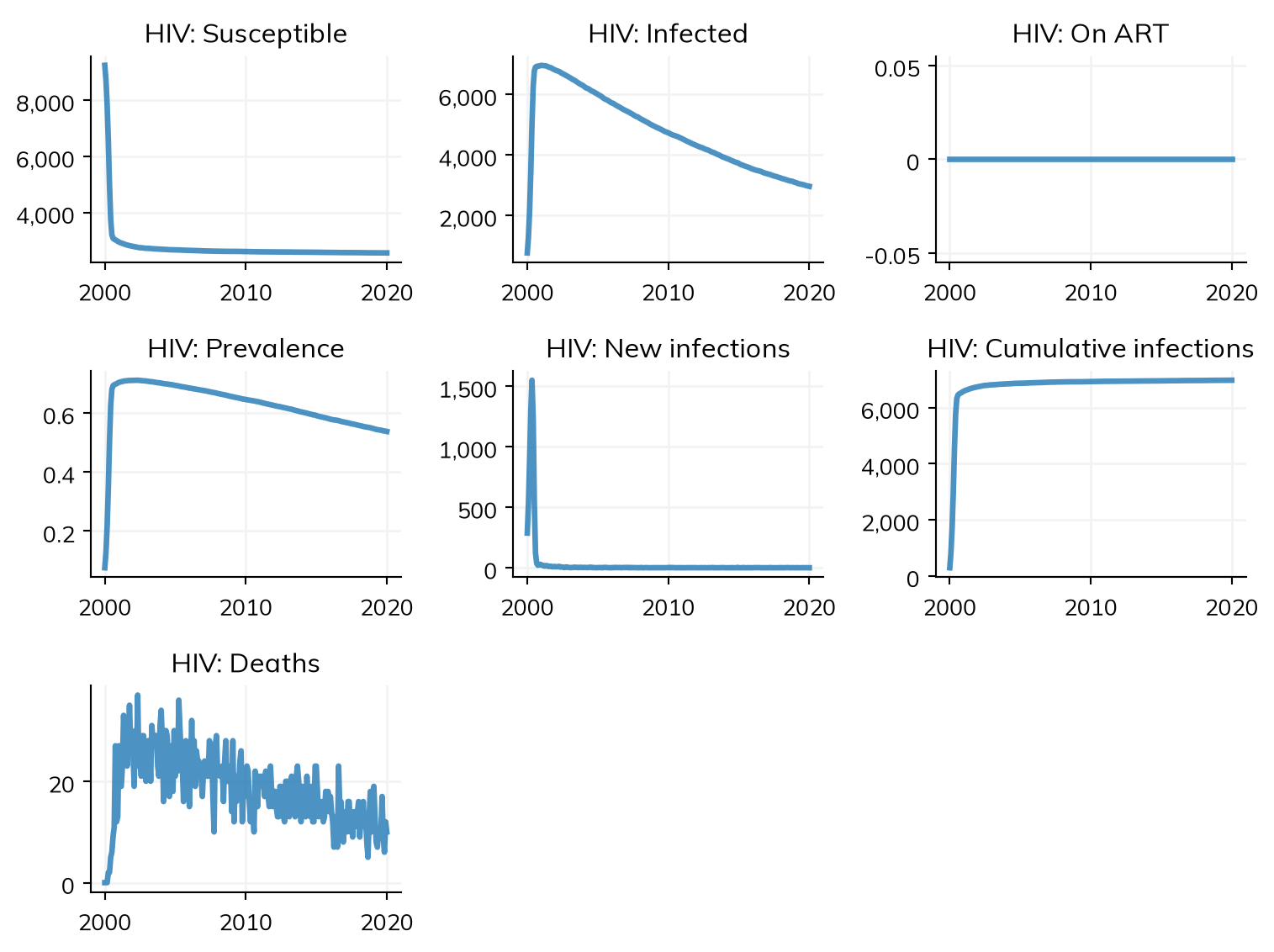
Q: Adapt the HIV example to include both MF and MSM transmission.
A: We add an ss.MSMNet alongside the ss.MFNet, and specify a beta for each network in the disease’s beta dictionary:
import starsim as ssimport starsim.library as ssl# HIV transmitting on both networkshiv = ssl.diseases.HIV(beta={'mf': [0.05, 0.025], 'msm': [0.08, 0.08]})# Heterosexual and MSM networksmf = ss.MFNet(duration=1/24, acts=80)msm = ss.MSMNet(duration=1/24, acts=80)pars =dict(start=2000, dur=20, dt=1/12, verbose=0)sim = ss.Sim(pars=pars, diseases=hiv, networks=[mf, msm])sim.run()sim.plot('hiv')
Figure(768x576)
Question 2
Q: Modify the age_mf network to have different age bins and mixing probabilities.
A: This exercise is open-ended and depends on the assortativity you want to model. The general approach is to override add_pairs() in a subclass of ss.MFNet (as sketched in the tutorial), and within it, choose partners using your own age-bin logic — for example, by binning agents by age and drawing partners preferentially from nearby bins. The Networks user guide shows worked examples of age-structured mixing, which is the most robust starting point.
Question 3
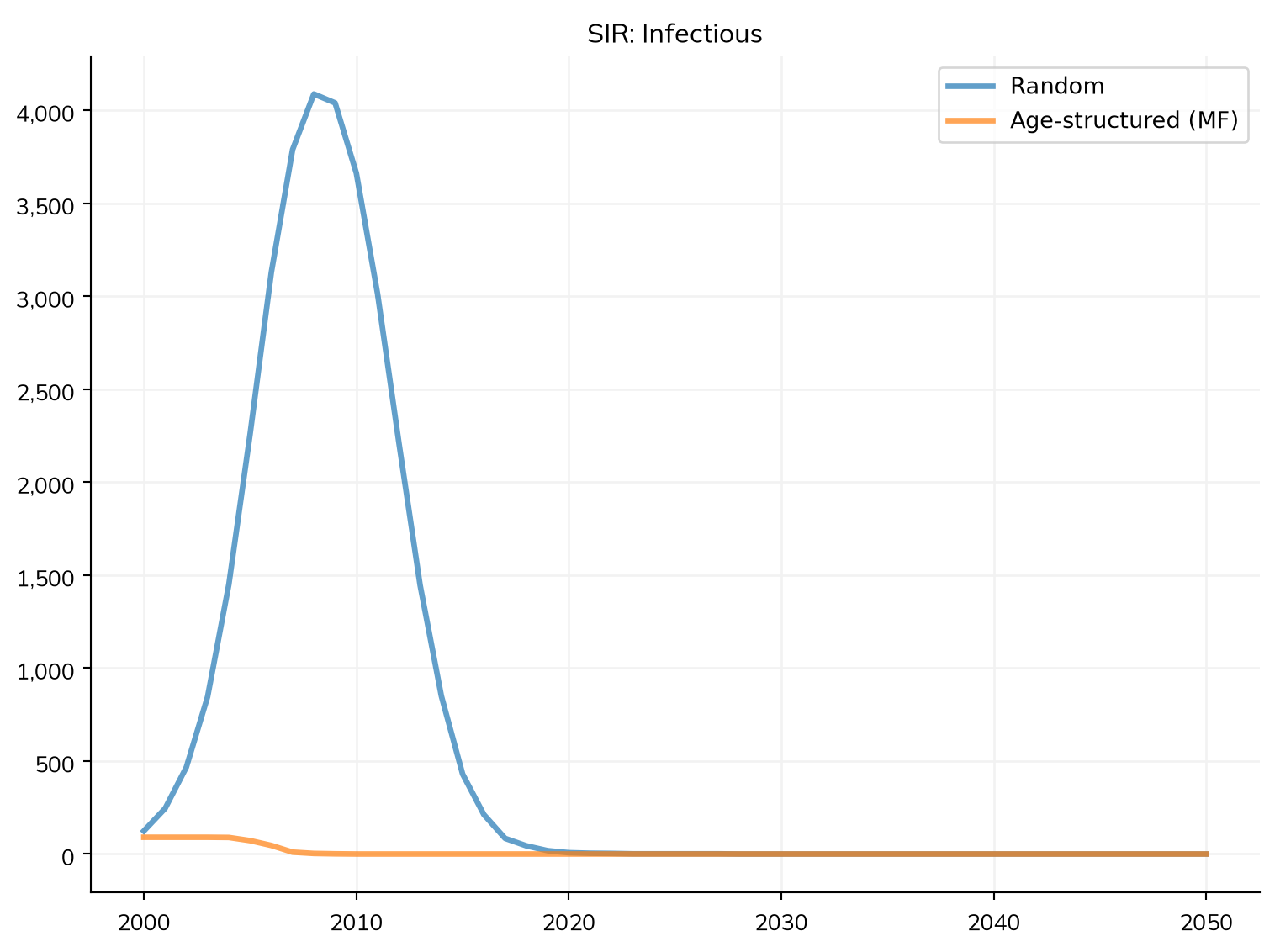
Q: Compare random vs age-structured networks — how do they affect epidemic dynamics?
A: We can run the same SIR disease on a structureless RandomNet and on the age-structured MFNet, and compare the infection trajectories:
The age-structured network restricts who can contact whom (and the MFNet only connects agents in partnerships), so it typically produces slower, smaller epidemics than a random network where every agent can mix freely.
T6 Solutions
Question 1
Q: If we change the disease from SIR to SIS and set coverage to 100%, what minimum efficacy of vaccine is required to eradicate the disease by 2050?
A: There are many ways we could solve this, including with formal numerical optimization packages. However, since we are only varying a single parameter, we can also just use a simple binay search or grid search. This solution illustrates both approaches.
import numpy as npimport sciris as scimport starsim as sspars =dict( n_agents =5_000, birth_rate =20, death_rate =15, networks =dict(type='random', n_contacts =4 ), diseases =dict(type='sis', dur_inf =10, beta =0.1, ), verbose =False,)class sis_vaccine(ss.Vx):""" A simple vaccine against "SIS" """def__init__(self, efficacy=1.0, **kwargs):super().__init__()self.define_pars(efficacy=efficacy)self.update_pars(**kwargs)returndef administer(self, people, uids): people.sis.rel_sus[uids] *=1-self.pars.efficacyreturndef run_sim(efficacy):""" Run a simulation with a given vaccine efficacy """# Create the vaccine product product = sis_vaccine(efficacy=efficacy)# Create the intervention intervention = ss.routine_vx( start_year=2015, # Begin vaccination in 2015 prob=1.0, # 100% coverage product=product # Use the SIS vaccine )# Now create two sims: a baseline sim and one with the intervention sim = ss.Sim(pars=pars, interventions=intervention) sim.run()return simdef objective(efficacy, penalty=10, boolean=False, verbose=False):""" Calculate the objective from the simulation """ sim = run_sim(efficacy=efficacy) transmission = sim.results.sis.new_infections[-1] >0if boolean:returnnot transmissionelse: loss = efficacy + penalty*transmissionif verbose:print(f'Trial: {efficacy=}, {transmission=}, {loss=}')return lossdef grid_search(n=5, reps=2):""" Perform a grid search over the objective function """ sc.heading('Performing grid search ...') lb =0# Lower bound for efficacy ub =1# Upper bound for efficacyfor rep inrange(reps):print(f'Grid search {rep+1} of {reps}...') efficacy = np.linspace(lb, ub, n) transmission = sc.parallelize(objective, efficacy, boolean=True) lb = efficacy[sc.findlast(transmission, False)] ub = efficacy[sc.findfirst(transmission, True)]print(f' Trials: {dict(zip(efficacy, transmission))}')print(f' Results: lower={lb}, upper={ub}') mid = (lb+ub)/2print(sc.ansi.bold(f'Result: {mid}'))return mid, lb, ubdef auto_search(efficacy=1.0):""" Perform automatic search """ sc.heading('Performing automatic search...') out = sc.asd(objective, x=efficacy, xmin=0, xmax=1, maxiters=10, verbose=True)print(sc.ansi.bold(f'Result: {out.x}'))return out# Run both optimizationsmid, lb, ub = grid_search()out = auto_search()