Parameter identification

The Starsim framework includes a built-in susceptible-infected-recovered (SIR) within-host progression module that can be used as a building block to developing more realistic agent-based models. Here, we use that SIR within-host module in combination with mixing pool transmission to create a simple SIR disease model.

Here, we use that SIR disease model to test two calibration workflows. The goal is to assess if they able to re-identify a known “true” set of parameters and explore the resulting latent trajectories. The two workflows demonstrated are: 1. Likelihood maximization using the optuna package as integrated with Starsim 2. Posterior sampling using a Bayesian workflow

Re-identifying the known parameter values from synthetic data provides reassurance that the calibration workflow is functioning as expected. For a more realistic Starsim calibration example, please see Calibration.

# Configure notebook autoreloading and inline plotting
%load_ext autoreload
%autoreload 2
%matplotlib inline

##%% Imports and settings
import numpy as np
import pandas as pd
import sciris as sc
import warnings
import optuna
import matplotlib.dates as mdates
import seaborn as sns
from IPython.display import display
import matplotlib.pyplot as plt
from scipy.special import betaln, gammaln
import starsim as ss

# Set additional options
optuna.logging.set_verbosity(optuna.logging.CRITICAL)
ss.options(jupyter=True)
warnings.simplefilter(action='ignore', category=FutureWarning)
warnings.filterwarnings('ignore', category=optuna.exceptions.ExperimentalWarning)

SIR model setup

First, we create a simple agent-based SIR simulation using Starsim.

def make_sim():
    """
    Make a simple SIR simulation using Starsim.

    Returns
    -------
    Sim
        A single simulation that has been configured, but not initialized or run.
    """
    sir_pars = dict(
        init_prev = 0.01, # Initial prevalence
        p_death = 0,      # No deaths
    )
    sir = ss.SIR(pars=sir_pars)

    net = ss.MixingPool(
        beta = 1,       # This is a multiplier on the disease beta
        n_contacts = 2, # Poisson lambda
    )

    sim_pars = dict(
        n_agents = 500,      # Number of agents in the simulation
        dt = ss.days(1),      # One-day time step
        start = '2025-01-01', # Start date of the simulation
        dur = 100,            # Duration of the simulation
        verbose = 0,          # Level of detail printed to the console
    )
    sim = ss.Sim(pars=sim_pars, diseases=sir, networks=net)
    return sim

def modify_sim(sim, calib_pars, rand_seed=0):
    """
    Modify the given simulation with the calibration parameters and random seed.
    
    Parameters
    ----------
    sim : Sim
        The simulation to modify.
    calib_pars : dict
        The calibration parameters to apply; note that the parameter values to use are stored in "value."
    rand_seed : int
        The random seed to use for the simulation.

    Returns
    -------
    Sim
        The modified simulation.
    """

    # Explicitly look for each of the calibration parameters and set the appropriate values
    if 'beta' in calib_pars:
        β = ss.perday(calib_pars['beta']['value']) # Use per-day for the transmission rate
        sim.pars.diseases.pars['beta'] = β

    if 'gamma' in calib_pars:
        γ = calib_pars['gamma']['value']
        sim.pars.diseases.pars['dur_inf'].set(1/γ)

    sim.pars['rand_seed'] = rand_seed

    return sim

def run_starsim(pars, rand_seed=0):
    """
    Run a Starsim SIR model with given parameters and random seed, returning results.

    Parameters
    ----------
    pars : dict
        The parameters dictionary with Optuna a values stored in "value."
    rand_seed : int
        The random seed to use for the simulation.

    Returns
    -------
    dataframe
        The results of the SIR model with columns of S, I, and R and index of Time.
    """
    # Make and modify the simulation
    sim = make_sim()
    sim = modify_sim(sim, pars, rand_seed)

    sim.run() # Run the simulation

    # Extract the results
    results = pd.DataFrame(dict(
        S = sim.results.sir.n_susceptible,
        I = sim.results.sir.n_infected,
        R = sim.results.sir.n_recovered,
    ), index=pd.Index(sim.results.timevec, name='Time'))
    results['rand_seed'] = rand_seed # Store the random seed for later reference

    return results

Calibration setup

We will calibrate two parameters, beta and gamma, each allowed to take on values between 0 and 1.

# Define the calibration parameters in a simple dictionary
calib_pars = dict(
    beta = {'low': 0, 'high': 0.15},
    gamma = {'low': 0, 'high': 0.08},
)

If using the optimization-based approach in Starsim, likelihood functions are defined and available for use. However, for the sampling-based approach, we will need to create our own likelihood.

def beta_binomial_likelihood(results, calib_data,
    kappa       = 10.0,
    prior_alpha = 1.0,
    prior_beta  = 1.0
):
    """
    Likelihood for Beta-Binomial observation model:
        s_obs ~ BetaBinomial(n_obs, alpha=kappa*p_hat, beta=kappa*(1-p_hat))
        p_hat is computed as (sim_x + prior_alpha) / (sim_n + prior_alpha + prior_beta).

    Parameters
    ----------
    results: DataFrame
        The results of a simulation.
    calib_data: DataFrame
        The calibration data to compare against.
    kappa: float
        Concentration parameter: larger values imply less over-dispersion.
    prior_alpha: float
        Prior alpha used to smooth the estimate of p_hat.
    prior_beta: float
        Prior beta used to smooth the estimate of p_hat.

    Returns
    -------
    float
        The likelihood of the observed data given the simulation results.
    """

    obs_x = calib_data['x'].values
    obs_n = calib_data['n'].values

    sim_x = results['I']
    sim_n = results.sum(axis=1)

    denom = np.maximum(sim_n + prior_alpha + prior_beta, 1e-12)  # guard
    p_hat = (sim_x + prior_alpha) / denom

    p_hat = np.clip(p_hat, 1e-9, 1 - 1e-9)
    alpha = kappa * p_hat
    beta  = kappa * (1.0 - p_hat)

    # log binomial coefficient: log C(n, x)
    logC = gammaln(obs_n + 1) - gammaln(obs_x + 1) - gammaln(obs_n - obs_x + 1)
    loglik = logC + betaln(obs_x + alpha, obs_n - obs_x + beta) - betaln(alpha, beta)
    return np.exp(np.sum(loglik)) # Exponentiated sum of logs

Bayesian calibration requires a prior distribution over the parameters. Here, we define a simple uniform prior over beta and gamma.

def sample_from_prior(size=1):
    """
    Sample beta and gamma from a uniform prior.

    Parameters
    ----------
    size : int
        Number of samples to draw.

    Returns
    -------
    Pandas DataFrame
        DataFrame of shape (size, 2) with columns [beta, gamma].
    """
    beta = np.random.uniform(calib_pars['beta']['low'], calib_pars['beta']['high'], size)
    gamma = np.random.uniform(calib_pars['gamma']['low'], calib_pars['gamma']['high'], size)

    return pd.DataFrame({'beta': beta, 'gamma': gamma})

Generate synthetic data for reidentification

That set the basic machinery of the SIR simulation model. Next, we’ll create some synthetic data to use as calibration targets. Because the model is stochastic, we’ll average over several replicates.

n_reps = 25 # Average over 25 repetitions to reduce stochastic noise

# These are the true parameters the optimizer will later try to identify
true_pars = dict(
    beta = dict(value=0.05),
    gamma = dict(value=0.03),
)

# Run the starsim SIR simulations in parallel.
# If you need to run in serial, for example when debugging, simply set serial=True
results_list = sc.parallelize(run_starsim, pars=true_pars, iterkwargs=dict(rand_seed=np.arange(n_reps)), serial=False)
results = pd.concat(results_list) # Combine the results into a single DataFrame
ave = results.groupby('Time').mean().drop(columns='rand_seed') # Average the results over the repetitions

# Extract synthetic data for calibration
observation_times = np.array([pd.Timestamp('2025-01-01')+pd.DateOffset(days=d) for d in [20, 40, 80]])
starsim_data = pd.DataFrame({
    'x': ave.loc[observation_times, 'I'].astype(int),
    'n': ave.loc[observation_times].sum(axis=1).astype(int),
    'Prevalence': ave.loc[observation_times, 'I'] / ave.loc[observation_times].sum(axis=1)
}, index=pd.Index(observation_times, name='t'))

print('Here is the data extracted from the average simulation to be used during calibration:\n')
display(starsim_data)

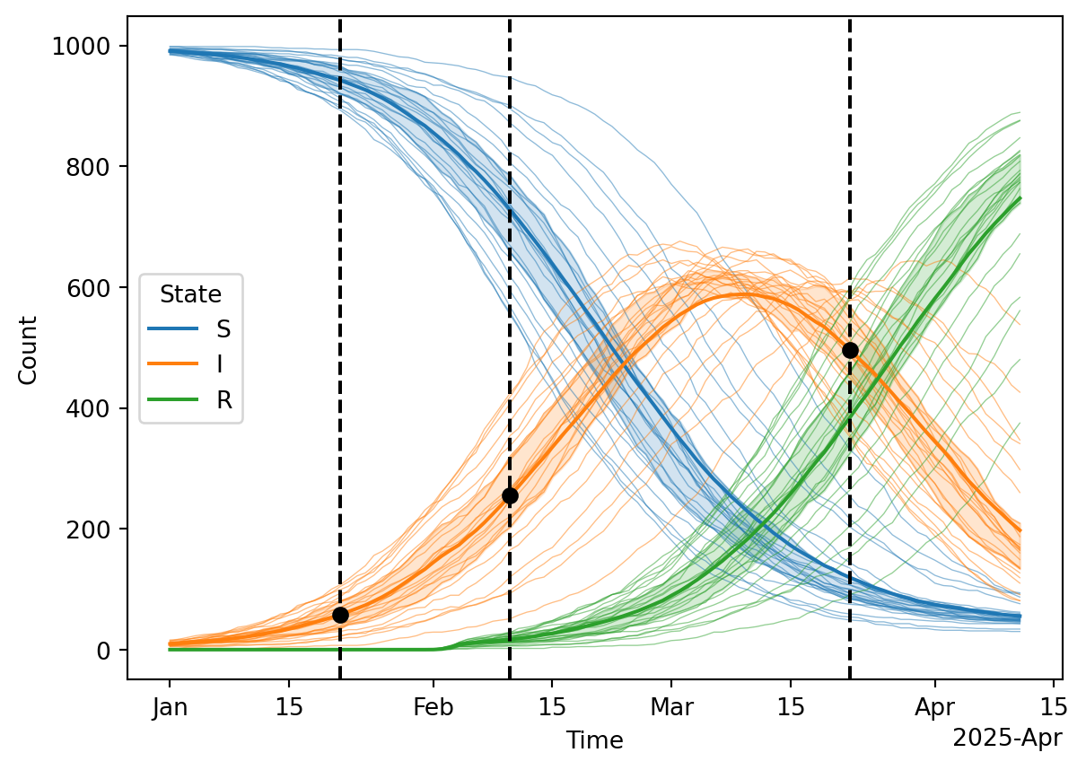
# Plot the results, vertical dashed lines indicate the observation times where prevalence is measured
df = results.reset_index().melt(id_vars=['Time', 'rand_seed'], value_vars=['S', 'I', 'R'], var_name='State', value_name='Count')
ax = sns.lineplot(data=df, hue='State', x='Time', y='Count', units='rand_seed', estimator=None, alpha=0.5, lw=0.5, legend=False)
sns.lineplot(data=df, hue='State', x='Time', y='Count', errorbar=('pi', 50), ax=ax, legend=True)
ax.xaxis.set_major_formatter(mdates.ConciseDateFormatter(ax.xaxis.get_major_locator()))
for ot in observation_times:
    ax.axvline(ot, ls='--', color='black')
ax.scatter(starsim_data.index, starsim_data['x'], marker='o', color='black', label='Observed data', zorder=10);

Here is the data extracted from the average simulation to be used during calibration:

	x	n	Prevalence
t
2025-01-21	29	500	0.05832
2025-02-10	118	500	0.23720
2025-03-22	246	500	0.49352

Likelihood maximization using the optuna package as integrated with Starsim

Starsim provides built-in integration with Optuna to make advanced model calibration easier. We demonstrate that linkage below using a Beta-binomial likelihood function.

sim = make_sim() # Begin by making a single "base" simulation with default parameters

# This example will use a single calibration component. We choose a
# Beta-binomial functional form to represent the "prevalence survey" data,
# taking advantage of both the numerator (x) and denominator (n) data.
prevalence_component = ss.BetaBinomial(
    name = 'SIR Disease Prevalence',

    # The starsim_data data has a date for each observation. The
    # "step_containing" conform method will extract simulation results on the
    # time step containing the observation date.
    conform = 'step_containing',

    # Here is the data we are trying to match, using the "x" and "n" columns
    # from the starsim_data DataFrame.
    expected = starsim_data[['x', 'n']],

    # And here is how we will extract the relevant data from the simulation results
    extract_fn = lambda sim: pd.DataFrame({
        'x': sim.results.sir.n_infected, # Numerator
        'n': sim.results.n_alive,        # Denominator
    }, index=pd.Index(sim.results.timevec, name='t')),
)

# Now make the calibration
calib = ss.Calibration(
    sim          = sim,                    # The base simulation
    calib_pars   = calib_pars,             # The calibration parameters
    build_fn     = modify_sim,             # The function to modify the base simulation with the calibration parameters
    reseed       = True,                   # Reseed the simulation for each calibration trial
    components   = [prevalence_component], # The calibration components
    total_trials = 100,                    # Total number of trials to run
    verbose      = False,                  # Shh...

    # Select and configure the sampler (optional)
    sampler = optuna.samplers.TPESampler(n_startup_trials=50)
)

calib.calibrate() # Let's go!

# Print out a summary
sc.colorize(color='blue', string=f'The best parameters identified by the optimization are:\n\
    * {calib.best_pars}\n\
    These parameters should be close to the true parameters:\n\
    * {true_pars}\n\
    The best parameters resulted in a loss of {calib.study.best_value}.')

The best parameters identified by the optimization are:

    * {'beta': 0.06724435254415136, 'gamma': 0.031111647022675555, 'rand_seed': 180749}

    These parameters should be close to the true parameters:

    * {'beta': {'value': 0.05}, 'gamma': {'value': 0.03}}

    The best parameters resulted in a loss of 4.112063381156048.

It seems like the best parameter values are pretty close to the right values, so that’s good. We can look at all the results and easily create a DataFrame containing the top K runs.

df = calib.to_df(top_k=10)
display(df)

	value	datetime_start	datetime_complete	duration	params_beta	params_gamma	params_rand_seed	state
number
58	4.112063	2026-03-03 05:56:54.377806	2026-03-03 05:56:54.789868	0 days 00:00:00.412062	0.067244	0.031112	180749	COMPLETE
93	4.122662	2026-03-03 05:56:58.498824	2026-03-03 05:56:58.902004	0 days 00:00:00.403180	0.067236	0.031329	103833	COMPLETE
61	4.133343	2026-03-03 05:56:54.790107	2026-03-03 05:56:55.208084	0 days 00:00:00.417977	0.063394	0.034627	225236	COMPLETE
57	4.190551	2026-03-03 05:56:54.370828	2026-03-03 05:56:54.779432	0 days 00:00:00.408604	0.065705	0.030025	170504	COMPLETE
62	4.445105	2026-03-03 05:56:54.800903	2026-03-03 05:56:55.218383	0 days 00:00:00.417480	0.063393	0.035096	234115	COMPLETE
98	4.548496	2026-03-03 05:56:58.989041	2026-03-03 05:56:59.321514	0 days 00:00:00.332473	0.066905	0.033322	206975	COMPLETE
95	4.749304	2026-03-03 05:56:58.605995	2026-03-03 05:56:59.018103	0 days 00:00:00.412108	0.061539	0.036619	260157	COMPLETE
73	4.931158	2026-03-03 05:56:56.412888	2026-03-03 05:56:56.824802	0 days 00:00:00.411914	0.062960	0.036354	283593	COMPLETE
65	5.158658	2026-03-03 05:56:55.218863	2026-03-03 05:56:55.670006	0 days 00:00:00.451143	0.063329	0.036457	235702	COMPLETE
64	5.237500	2026-03-03 05:56:55.054557	2026-03-03 05:56:55.496375	0 days 00:00:00.441818	0.066450	0.035877	236642	COMPLETE

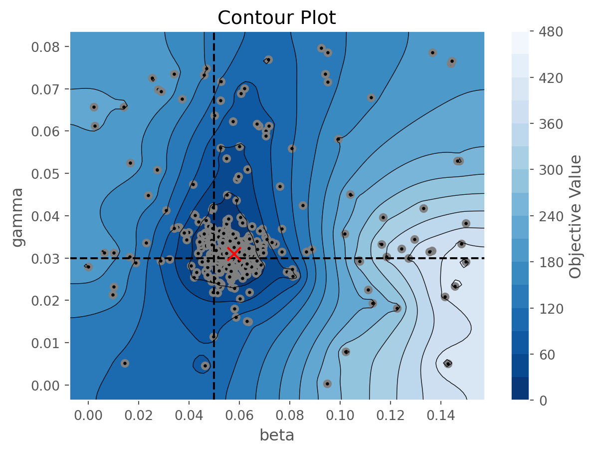
# Plot the results
figs = calib.plot_optuna(['plot_optimization_history', 'plot_contour'])
figs[0].axes.set_yscale('log')

figs[1].axvline(true_pars['beta']['value'], ls='--', color='black')
figs[1].axhline(true_pars['gamma']['value'], ls='--', color='black')
figs[1].scatter(calib.study.best_params['beta'], calib.study.best_params['gamma'], 100, marker='x', color='red', zorder=10);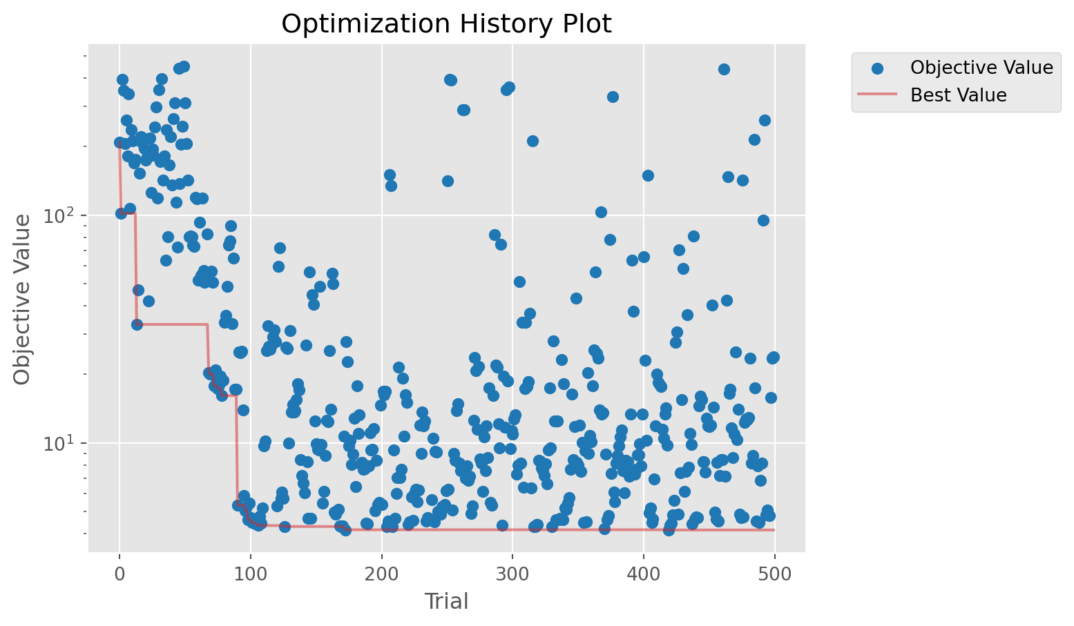

Finally, let’s run some simulations with the best parameters and compare to the calibration data. From a mathemtatical perspective, this is not the right thing to do. We have found the maximum-likelihood estimate (MLE) parameters, \(\theta\), and are now running simulations \(X \mid \theta\). These latent state trajectories represent the intrinsic noise in the model, but do not represent uncertainty. For that, additional methods are required or use a Bayesian approach, as illustrated below.

n_reps = 10 # Number of repetitions to run

# These are the best parameters found, the MLE estimate
best_pars = dict(
    beta = dict(value=calib.study.best_params['beta']),
    gamma = dict(value=calib.study.best_params['gamma']),
)

# Run the starsim SIR simulations in parallel, cool! If you need to run in
# serial, for example when debugging, simply set serial=True
results_list = sc.parallelize(run_starsim, pars=best_pars, iterkwargs=dict(rand_seed=np.arange(n_reps)), serial=False)
results = pd.concat(results_list) # Combine the results into a single DataFrame

# Plot the results, vertical dashed lines indicate the observation times where prevalence is measured
df = results.reset_index().melt(id_vars=['Time', 'rand_seed'], value_vars=['S', 'I', 'R'], var_name='State', value_name='Count')
ax = sns.lineplot(data=df, hue='State', x='Time', y='Count', units='rand_seed', estimator=None, alpha=0.5, lw=0.5, legend=False)
sns.lineplot(data=df, hue='State', x='Time', y='Count', errorbar=('pi', 50), ax=ax, legend=True)
ax.xaxis.set_major_formatter(mdates.ConciseDateFormatter(ax.xaxis.get_major_locator()))
for ot in observation_times:
    ax.axvline(ot, ls='--', color='black')
ax.scatter(starsim_data.index, starsim_data['x'], marker='o', color='black', label='Observed data');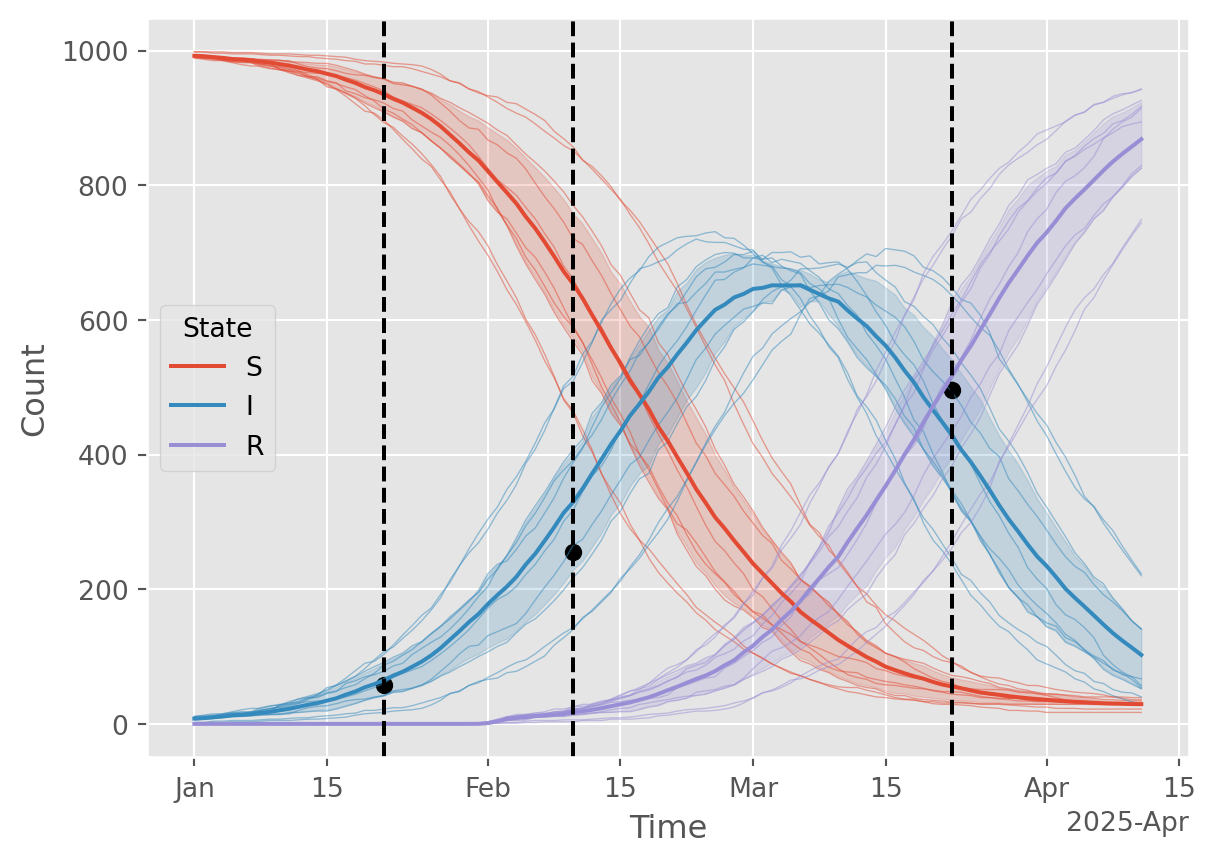

Bayesian calibration using sampling-importance resampling (SIR)

Now let’s use a Bayesian calibration approach to see if the results are any different. We’ll use a simple ABC rejection sampling with a beta-binomial likelihood. A key difference is that we’re learning a posterior distribution over both parameters and trajectories rather than just a point estimate of the parameters.

N = 100  # Number of prior samples (more is better, but slower)
# For Beta-Binomial, the concentration parameter. Lower kappa --> broader
# posterior and higher effective sample size (ESS) for the same N. But not a
# free parameter, kappa comes from the over-dispersion in the observed data.
kappa = 10 

# Sample from the prior
prior_samples = sample_from_prior(size=N)

rand_seeds = np.random.randint(0, 1e6, size=2*N)
rand_seeds = np.unique(rand_seeds)[:N]

# Prepare parameter dicts for each sample
sample_pars_list = [
    {
        'pars': {'beta': {'value': row['beta']}, 'gamma': {'value': row['gamma']}},
        'rand_seed': rand_seeds[idx]  # Random seed for each simulation
    }
    for idx, row in prior_samples.iterrows()
]

# Run simulations in parallel and collect trajectories
sim_results_list = sc.parallelize(run_starsim, iterkwargs=sample_pars_list, serial=False)

# Store latent state trajectories for each sample
trajectories = pd.concat(sim_results_list) \
    .reset_index() \
    .set_index(['rand_seed', 'Time'])

# Compute likelihoods for each sample
likelihoods = []
for rand_seed, sim_result in trajectories.groupby('rand_seed'):
    sim_sir = sim_result.loc[rand_seed].loc[observation_times, ['S', 'I', 'R']]
    likelihood = beta_binomial_likelihood(sim_sir, starsim_data, kappa=kappa)
    likelihoods.append((rand_seed, likelihood))

results = pd.DataFrame(likelihoods, columns=['rand_seed', 'likelihood'])
results = pd.concat([prior_samples, results], axis=1).set_index('rand_seed')

Within a Bayesian workflow, there are two ways to proceed from this point. 1. Use all samples, weighted by their likelihood. For this approach, there is no resampling step. 2. Resample \(K \leq N\) samples with probability proportional to their likelihood (with replacement). This is sampling-importance resampling (SIR), not to be confused with the susceptible-infected-recovered (SIR) model. Ideally, we would choose \(K=N\) resamples, but if using these samples for further analysis, it may be useful to choose \(K < N\) to reduce computational cost. It’s generally recommended to choose \(K\) as one to two times the effective sample size (ESS).

results['weight'] = results['likelihood'] / np.sum(results['likelihood'])

# Importance resampling
ESS = 1 / np.sum(results['weight']**2)
print('='*60)
print(f'Effective Sample Size (ESS) = {ESS:.1f} out of {N}')
if ESS < 30:
    print('WARNING: ESS is below 30, consider increasing N')
print('='*60)


K = np.ceil(1.5 * ESS).astype(int)  # Number of samples to draw
print('Resampling K =', K, 'samples from the weighted ensemble of N =', N, 'samples')
resample_seeds = np.random.choice(results.index, size=K, replace=True, p=results['weight'])

# Merge results into combined (all) and selected (K<N subset)
combined = trajectories.reset_index().merge(results, on='rand_seed').set_index(['rand_seed', 'Time'])
selected = combined.loc[resample_seeds]

# Show posterior samples as a DataFrame
posterior_pars = results.loc[resample_seeds, ['beta', 'gamma']]
display(posterior_pars.head())

============================================================
Effective Sample Size (ESS) = 10.4 out of 100
WARNING: ESS is below 30, consider increasing N
============================================================
Resampling K = 16 samples from the weighted ensemble of N = 100 samples

	beta	gamma
rand_seed
298521	0.034424	0.004403
102494	0.026410	0.024397
244801	0.030173	0.012495
35477	0.045826	0.040221
244801	0.030173	0.012495

Let’s look at the parameters, full (weighted) posterior mean, and posterior mean from the resample.

fig, ax = plt.subplots(figsize=(7, 6))

# Scatter all prior samples, colored by likelihood
scat = ax.scatter(
    results['beta'], results['gamma'],
    c=results['weight'], cmap='viridis', s=15, edgecolor='none', alpha=0.8
)

# Overlay red rings for the K resampled posterior samples
ax.scatter(
    results.loc[resample_seeds, 'beta'], results.loc[resample_seeds, 'gamma'],
    facecolors='none', edgecolors='red', s=25, linewidths=1, label='Resampled'
)

# Overlay the true parameter values and best posterior sample
ax.axvline(true_pars['beta']['value'], ls='--', color='black', label='True parameters')
ax.axhline(true_pars['gamma']['value'], ls='--', color='black')

# Mark the full and resampled posterior means
full_posterior_mean = results[['beta', 'gamma']].T.dot(results['weight'])
ax.scatter(full_posterior_mean.beta, full_posterior_mean.gamma, 100, marker='x', color='red', lw=2, zorder=10, label='Posterior mean (full)')
posterior_mean = results.loc[resample_seeds, ['beta', 'gamma']].mean(axis=0)
ax.scatter(posterior_mean.beta, posterior_mean.gamma, 100, marker='x', color='blue', lw=2, zorder=11, label='Posterior mean (resampled)')

ax.set_xlabel('beta')
ax.set_ylabel('gamma')
ax.set_title('Posterior parameter samples (red rings) and prior samples (colored by likelihood)')
plt.colorbar(scat, ax=ax, label='Normalized likelihood')
# Move the legend outside the figure to the right
plt.legend()
plt.tight_layout()
plt.show()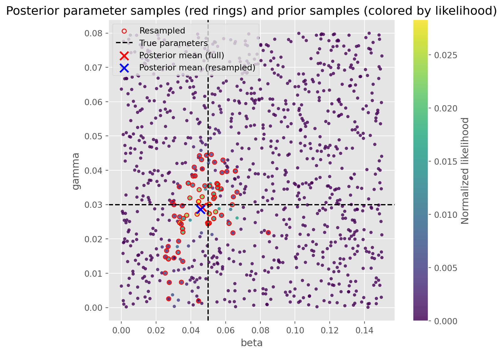

View latent trajectories based on all \(N\) samples, weighted by their likelihood. Takes some code to incorporate the weights into the plotting…

# Use ALL samples, with weights, to compute mean and quantiles
df = combined \
    .reset_index() \
    .melt(
        id_vars=['Time', 'rand_seed'],
        value_vars=['S', 'I', 'R'],
        var_name='State',
        value_name='Count'
    )
df['Weight'] = df['rand_seed'].map(results['weight']) # Add weights to the DataFrame

def weighted_quantile(values, quantiles, weights):
    v = np.asarray(values, float)
    q = np.atleast_1d(quantiles).astype(float)
    w = np.asarray(weights, float)
    order = np.argsort(v)
    v, w = v[order], w[order]
    cw = np.cumsum(w)
    cw /= cw[-1] if cw[-1] > 0 else 1.0
    return np.interp(q, cw, v)

def summarize(group):
    vals = group['Count'].to_numpy()
    wts  = group['Weight'].to_numpy()
    mean = np.average(vals, weights=wts)
    q05, q25, q75, q95 = weighted_quantile(vals, [0.05, 0.25, 0.75, 0.95], wts)
    return pd.Series({'mean': mean, 'q05': q05, 'q25': q25, 'q75': q75, 'q95': q95})

summary = (
    df.groupby(['Time','State'], sort=True, as_index=False)
      .apply(summarize)
      .reset_index(drop=True)
)

fig, ax = plt.subplots(figsize=(9,5))
lines = sns.lineplot(data=summary, x='Time', y='mean', hue='State', hue_order=['S', 'I', 'R'],
                     estimator=None, errorbar=None, ax=ax, zorder=5)

# Get the colors used by seaborn for each state
state_colors = {line.get_label(): line.get_color() for line in ax.lines}

for state, g in summary.groupby('State'):
    color = state_colors.get(state, None)
    ax.fill_between(g['Time'], g['q05'], g['q95'], alpha=0.12, linewidth=0, color=color)  # 90% band
    ax.fill_between(g['Time'], g['q25'], g['q75'], alpha=0.25, linewidth=0, color=color)  # 50% band

for ot in observation_times:
    ax.axvline(ot, ls='--', color='black')
ax.scatter(starsim_data.index, starsim_data['x'], marker='o', color='black', label='Observed data', zorder=10);

ax.set_ylabel('Count')
ax.set_title('Weighted posterior trajectories')
ax.legend(title='State')
ax.xaxis.set_major_formatter(mdates.ConciseDateFormatter(ax.xaxis.get_major_locator()))
plt.tight_layout()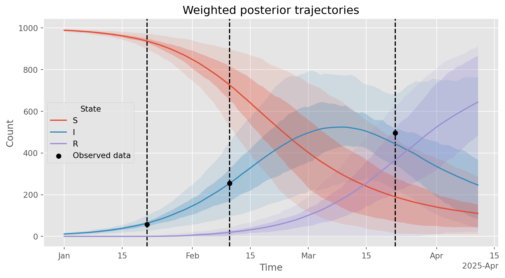

# Plot the resampled trajectories. Should be similar to the weighted posterior over latent trajectories shown above.
df = selected \
    .reset_index() \
    .melt(
        id_vars=['Time', 'rand_seed'],
        value_vars=['S', 'I', 'R'],
        var_name='State',
        value_name='Count'
    )

fig, ax = plt.subplots(figsize=(9,5))
sns.lineplot(data=df, hue='State', x='Time', y='Count', units='rand_seed', estimator=None, alpha=0.5, lw=0.2, legend=False, ax=ax)
sns.lineplot(data=df, hue='State', x='Time', y='Count', errorbar=('pi', 50), alpha=0.5, ax=ax, legend=True, zorder=5)
sns.lineplot(data=df, hue='State', x='Time', y='Count', errorbar=('pi', 90), alpha=0.25, ax=ax, legend=False, zorder=6)
ax.xaxis.set_major_formatter(mdates.ConciseDateFormatter(ax.xaxis.get_major_locator()))
for ot in observation_times:
    ax.axvline(ot, ls='--', color='black')
ax.scatter(starsim_data.index, starsim_data['x'], marker='o', color='black', label='Observed data', zorder=10);
ax.legend(title='State')
ax.set_title('Resampled posterior trajectories')
plt.tight_layout()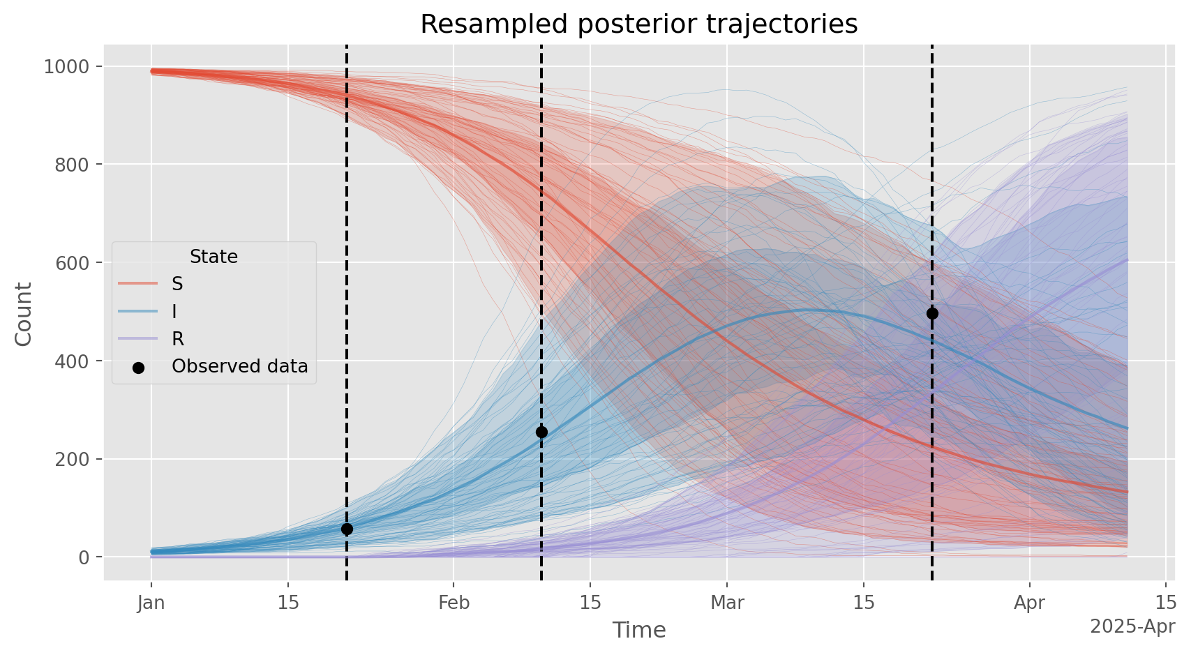

The next step would be scenario analysis using these \(K\) resamples parameters and latent trajectories. Each of these \(K\) samples represents a different possible future trajectory of the epidemic, and the ensemble of these \(K\) trajectories can be used to quantify uncertainty in future projections. Each of these \(K\) trajectories should be simulated forward \(M\) times for each scenario, using common random numbers, to produce final results.